Artículo

 

Development of Barostats for Finite Systems Born-Oppenheimer Molecular Dynamics Simulations

 

Gabriel Ulises Gamboa,¹* Patrizia Calaminici and Andreas M. Köster

 

¹ Departamento de Química, CINVESTAV, Avenida Instituto Politécnico Nacional 2508, A.P. 14-740 México D.F. 07000, México. pcalamin@cinvestav.mx, akoster@cinvestav.mx

² Present Address: Department of Physics, Virginia Commonwealth University, Richmond, Virginia 23284. gugamboamart@vcu.edu

 

Received November 29, 2011.
Accepted April 02, 2012.

 

Abstract

A new method for pressure control in first-principle molecular dynamics simulations for finite systems is presented. The extended Lagrangian methodology is applied to generate the equations of motion and the system's volume is obtained by a purely geometrical procedure, which is inexpensive in terms of computational cost. The implementation of all discussed algorithms was carried out in the program deMon2k where a robust machinery for auxiliary density functional theory calculations exists. The here described methodology extend our effort on property calculations beyond the polyatomic ideal gas approximation on the basis of first-principle electronic structure calculations.

Key words: Molecular Dynamics, Finite Systems, Barostats.

 

Resumen

Se presenta un nuevo método para controlar la presión en simulaciones de dinámica molecular de primeros principios. La metodología del Lagrangiano extendido es aplicada para la generación de las ecuaciones de movimiento y el volumen del sistema se obtiene de un procedimiento puramente geométrico, el cual es económico en términos de costo computacional. La implementación de los algoritmos discutidos se llevó a cabo en el programa deMon2k, donde existe una maquinaria robusta para cálculos de teoría de funcionales de la densidad auxiliar. La metodología aquí descrita amplía nuestro esfuerzo en cálculos de propiedades más allá de la aproximación del gas ideal con base en cálculos de estructura electrónica de primeros principios.

Palabras clave: Dinámica molecular, sistemas finitos, barostatos.

 

Introduction

Molecular Dynamics (MD) simulations are used to study the natural time evolution of a system of N particles in a volume V. In such simulations the total energy E is a constant of motion. The integration of the (classical) equations of motion for such a system leads, in the limit of infinite sampling, to a trajectory which maps onto a microcanonical (NVE) ensemble of microstates. Application of pressure to a given system may lead to electronic structure changes which will also modify the properties of the system. Many experimental measurements are made under constant temperature and pressure conditions, and thus, simulations in the isothermal-isobaric (NPT) ensemble can be most directly related to experimental data.

Although thermodynamic results can be transformed between ensembles, this is only reliable in the limit of infinite system size (the thermodynamic limit). In the case of molecules it may, therefore, be desirable to perform simulations in a specific ensemble. NPT simulations of bulk materials have been performed since the eighties, mainly due to the development of extended Lagrangians [1-6]. There, the volume of the system is well defined and identical to that of the simulation cell. The volume and the external pressure, as its conjugate variable, are included in the Lagrangian as a PV term. An artificial kinetic energy corresponding to the cell fluctuations is also introduced and the cell is treated as a dynamical variable, allowing the molecular dynamics trajectory to sample the NPT ensemble. These techniques have been applied to different systems and excellent agreements between experiment and theoretical simulations were found [7-9]. On the other hand, pressure control for finite systems is much less explored. Recent experiments of finite systems under pressure, such as clusters, nano-crystals, proteins and biological systems [10-28], have stimulated the interest in finite system barostats.

There are two main approaches to control the pressure in MD simulations of finite systems. The first one is based on the thermodynamic description of pressure as the result of (linear) momentum exchange between a particle and its environment. Here the environment can consist of different types of other particles or a container. In this treatment, a molecule is immersed into a classical repulsive fluid, with classical interactions between the molecule and the fluid. The parameters are chosen such that there is a clear volume partition between the two systems, and no fluid particle is allowed to be inside the simulated molecule. The whole system, liquid and molecule, is simulated at constant volume conditions. The fluid behaves as a pressure reservoir, equilibrating its pressure with the molecule's internal pressure. This approach is closed to experiment, where a finite system is in contact with a gas or a fluid. The pressure then depends on the fluid density and temperature. From a practical point of view, a certain drawback of the reservoir method is the necessity to use a relatively large number of fluid particles in order to avoid crystallization [29-30]. The second approach is based on the extended Lagrangian formalism where the pressure is taken into account by including a PV term in the description of the system. The Lagrangian for a system under external pressure P_ext then reads:

Where the terms on the right side represent the kinetic energy, potential energy and mechanical work on the system, respectively.

In this approach there is no need for an auxiliary liquid to exert pressure on the molecule. However, due to the lack of periodic boundary conditions, the volume of the system (V) is not imposed by the simulation cell but has to be calculated as a function of the atomic coordinates (R).

For this reason, considerable emphasis has been placed upon accurate calculations of the volume of molecules within the last years. Sun et al. [31] defines the total volume of the system as a sum of individual atomic volumes. Landau [32] estimates the volume based on the average inter-particle distance. Cococcioni et al. [33] have introduced a definition based on the quantum volume enclosed by a charge isosurface, and Calvo and Doye [34] have proposed a volume definition by finding the minimal polyhedron enclosing the finite system. Other definitions are based on an isotropic approximation to the finite system volume, e.g. by replacing the system by a sphere of a given radius, which is calculated from a combination of atomic coordinates [35]. Our work contributes to the second approach, i.e. the extended Lagrangian formalism. After a brief introduction of Born-Oppenheimer molecular dynamics employing auxiliary density functional theory (ADFT) [36] in the next section we introduce a simple, yet exact, volume definition for finite systems in Section 3. The computational details are given in Section 4. The results of our validation calculations are discussed in Section 5. Concluding remarks are drawn in the last section.

 

Born-Oppenheimer Molecular Dynamics with ADFT

In a full description of the energetics and dynamics of a system, all particles, which in our case are electrons and nuclei, should be treated quantum mechanically. However, for chemical studies, physical and practical considerations motivate calculations within the Born-Oppenheimer (BO) approximation [37]. This approximation introduces a separation of the time scales for the nuclear and electronic motions. It is at this level of approximation that the fundamental chemical concept of a molecular structure appears in the description of matter. To further simplify the equations of motion for the elementary particles we apply in our implementation the classical equations of motion for the propagation of the nuclei. Therefore, a BOMD step as discussed in this article consists of solving the static electronic structure problem, i.e. to solve the stationary Kohn-Sham equations [38], and the propagation of the nuclei via classical molecular dynamics. The resulting BOMD method is defined by:

Where Ĥ_KS, ψ(r) and e are the Kohn-Sham Hamiltonian, orbitals and their eigenvalues respectively, M_A stands for the mass of the atom A, Ä denotes its acceleration and E_pot is the potential energy function of the system. In the above described BOMD step, the solution of the Kohn-Sham equations (2) represents the computational bottleneck. In the framework of a localized basis set approach this task requires the calculation of 4-center electron repulsion integrals (ERIs). This calculation scales formally with the 4^th power of the size of the basis set, therefore, the size of treatable systems is severely limited by this step. The use of the variational fitting of the Coulomb potential approximation from Dunlap [39], reduces the scaling of the ERI calculation by one order because only 3-center integrals have to be calculated. For this purpose a second function set is introduced, the so called auxiliary function set. In the program deMon2k [40] the density calculated from this auxiliary function set is also used for the calculation of the exchange-correlation potential. This approach is named auxiliary density functional theory (ADFT) in the literature [36]. Here the molecular orbitals of a system are represented by a linear combination of Gaussian type orbitals and the auxiliary functions are represented by primitive Hermite Gaussian functions which share the same exponents within a set. Whereas the Kohn-Sham density scales quadratically with the number of basis functions, the auxiliary density scales only linearly with the number of auxiliary functions. This represents a considerable reduction in the grid work. Equations of motion (3) can be integrated with the velocity Verlet algorithm [41, 42], which yields a good compromise between accuracy and computational cost [43]. This performance opens then the possibility of computing molecular properties as a function of time with first-principle methods up to the nanosecond time scale [44].

 

Volume Definition for Finite Systems

In localized atomic orbital electronic structure methods a natural volume definition is obtained by the radial cutoffs of basis functions used in the analytical and numerical molecular integral calculations. Based on these cutoffs a spherical volume can be assigned to each atom. The radii of these atomic spheres are defined by the most diffuse basis functions at the atoms. Thus, the atomic volumes depend from the basis set of the atom and the basis function cutoff value, τ_V. Once the atomic volumes are calculated the molecular volume is obtained by the superposition of the atomic spheres. Inspired by the GEPOL program [45] we implemented a geometrical procedure for the molecular volume calculation. The algorithm can be summarized by the following steps:

1. Each atom, centered in A, is surrounded by a sphere with radius R_A calculated according to the (radial) basis function cutoff value, τ_V.

2. Each sphere is then divided into 60 spherical triangles of equal area. This is equivalent to the projection of a pentakisdodecahedron (Figure 1, left) on each sphere.

Now the tessellation is increased. Each initial triangular tesserae is divided into four triangles (Figure 1, right). Let x₁ and x₂ be the coordinates of two vertexes of the initial triangle. Then x_c is the coordinate corresponding to the midpoint along the chord (straight line passing by x₁ and x₂) calculated as:

This calculation is repeated for all sides of the 60 triangles. Please note that new x_C coordinates are not lying on the surface of the sphere (see Figure 2, left).

3. Calculation of the coordinates x_m of the vertexes of the new triangles on the sphere as depicted in Figure 2. These coordinates correspond to the midpoint along the arc on the sphere surface and are given by:

Here R_c is the distance from the origin of the sphere to x_c. By repeating this calculation for all x_c one obtains a set of 240 spherical triangles per sphere.

4. Steps 3 and 4 are repeated until the division process has yielded 3840 spherical triangles per sphere (atom).

5. Calculation of the center coordinates {x_n} for each spherical triangle. This procedure requires the calculation of the triangle's barycenter x_b (see Figure 3, left), given by:

where x_i, x_j and x_k stands for the vertexes after complete tessellation. The coordinates of the triangle center on the spherical surface (see Figure 3, right) are then the components of the vector:

6. Elimination of all triangles contained within the molecular surface, such that the remaining spherical triangles now form the envelope surface. The distance between the center of a triangle and the center of another sphere to which the triangle does not belong is calculated as |A - x_n| (see Figure 4, left). If this distance is less or equal to the radius of this sphere, i.e. |A - x_n| ≤ R_A, the triangle is discarded. This step is repeated with all spheres to which the triangle does not belong to. If the triangle is not discarded in this loop it belongs to the envelope surface. This process is repeated for all triangles forming the spherical surfaces.

7. Calculation of the molecular volume by summing all solid volumes spanned by the triangular surfaces and the origin of each sphere as depicted in Figure 4 (right). The molecular volume is given by:

Where a_i(A) is the area of the i^th triangle belonging to the sphere of atom A given by:

Here n_t denotes the number of triangles (3840) on each atomic sphere. In this way, the volume for molecules is calculated by a purely geometrical procedure, which in terms of computational cost is not expensive and has been applied already to biomacromolecules [45].

Once the molecular volume is defined the equations of motion for an isothermal-isobaric ensemble [46,47] can be formulated. Here we give these equations for a system of N particles coupled to a Nosé-Hoover chain thermostat [48-50] with n links and a barostat:

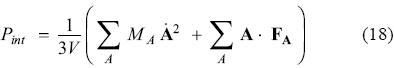
Here A, b and t, represent the positions of the atoms and the corresponding variables for the barostat and thermostat, respectively. The associated momenta are denoted by p_A, p_b and p_t. The dot on top of variables indicate first derivative with respect to time. N_f represents the number of degrees of freedom in the real system, V is the calculated volume, T₀ is the temperature of the bath, P_ext is the external (applied) pressure and P_int is the instantaneous (internal) pressure of the system, calculated as:

The thermostat "mass" parameters, m_ti, are related to the characteristic frequency of the motion of the particles, ω, by:

The barostat "mass" parameter, m_b, is defined as:

Here ω_b represents the coupling frequency between the barostat, the particles and the thermostat. The equations of motion (10)-(17) are integrated with the velocity Verlet algorithm, which requires the inversion of a (37V + n + 1)² matrix at least 2 times every time step.

 

Computational Details

The performance of the described methodology was tested with BOMD simulations for a water molecule running 50,000 steps with a step size of 0.2 fs. The local density approximation employing the exchange functional from Dirac [51] in combination with the correlation functional proposed by Vosko, Wilk and Nusair [52] was used. The target temperature was 500 K in all cases controlled by a Nosé-Hoover chain thermostat with 3 chain links with a coupling frequency of 1500 cm^-1. The target pressure was 10 atm using the here described methodology. All calculations were performed in the framework of ADFT with the double-Z valence polarization basis set and A2 auxiliary function set [53].

 

Results and Discussion

In the first set of validation calculations we varied the basis function cutoff value, τ_V, used for the calculation of the molecular volume. In these calculations τ_V was set to 10^-10 a.u., 10^-20 a.u. and 10^-30 a.u. and the barostat coupling frequency was fixed to 1500 cm^-1. Figure 5 depicts the average temperature and pressure profiles of these runs. As this figure shows the basis function cutoff value affects critically the BOMD pressure. For the here aimed pressure of 10 atm a τ_V of 10^-20 a.u. yields best results. The other cutoff values fail to equilibrate to the target pressure of 10 atm. However, the pressure stabilizes also in these runs. With τ_V = 10^-10 a.u. the equilibrated pressure stabilizes around 50 atm whereas it stabilizes around 1 atm with a cutoff value of 10^-30 a.u. as Figure 5 shows. This indicates that the basis set cutoff value must be chosen according to the target pressure. This is particularly critical for small pressures below 100 atm. Figure 5 also shows that the pressure equilibration is usually faster than the temperature equilibration. Therefore, it is recommended to first adjust the basis set cutoff values in NPT BOMD simulations with the here proposed methodology. Once this cutoff value is chosen it usually will work successfully for a large range of different temperatures. While temperature is controlled by a chain of thermostats, where each chain link acts as a particle buffering kinetic variables, the pressure control is driven by only one direct interacting quasi-particle, making temperature equilibration slower than pressure equilibration. In the here discussed examples all three calculations reach the target temperature in about 10 ps independent of the equilibrated pressure.

In a second set of validation calculations the basis function cutoff value, τ_V, was fixed to 10^-20 a.u. and the barostat coupling frequency was varied (500 cm^-1, 1500 cm^-1 and 3000 cm^-1). In Figure 6 the corresponding average temperature and pressure profiles are depicted. As can be seen from this figure the target pressure of 10 atm is obtained in all three runs independently of the barostat coupling frequency. Pressure equilibration is similar, however, best for the run with ω_b = 3000 cm^-1. The barostat frequency mainly affects temperature equilibration. In our case here the low frequency run (weak barostat coupling) slightly accelerates temperature equilibration.

Our validations shows that pressure control in finite systems can be realized with the here proposed parameter free volume definition. However, the described extended system barostat is sensible to the choice of the basis set cutoff value, τ_V. Because of the relative short time for pressure equilibration, a suitable τ_V value can be found in advance to the NPT simulation. Once this value is determined NPT and NVT simulations are very similar. In particular, the here proposed volume definition does not deteriorate the computational performance of our BOMD implementation. The thermostat coupling to the molecule is similar as in NVT simulations where no barostat is used. The here described methodology allows NPT simulations of finite systems as required for molecular phase diagram calculations.

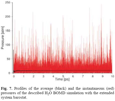
Figure 7 depicts the behavior of the instantaneous and average pressure of the performed BOMD simulation. The pressure fluctuations are usually much larger than the total energy fluctuations in a NVE simulation. This is expected because the pressure is related to the product of the positions and the position derivatives of the potential energy function, i.e. the forces. This product, A · F_A, changes faster with A than does the internal energy, hence the greater fluctuation in the pressure.

 

Conclusions

In this contribution we describe a new method for pressure control in first-principle molecular dynamics simulations for finite systems based on the extended Lagrangian methodology. The volume is defined via the basis function cutoff value, τ_V, of the atom centered basis set. It is calculated highly efficient by an analytical geometrical procedure. Our validation calculations show that the main adjustable parameter for pressure control is the basis function cutoff value. Because pressure equilibration is rather fast this value can be easily adjusted in short time test runs. Once the basis function cutoff value is adjusted the barostat behaves very stable in NPT simulations. With this implementation in deMon2k first-principle calculations of finite systems phase diagrams become possible.

 

Acknowledgements

G.U. Gamboa gratefully acknowledges a CONACyT Ph.D. fellowship (200113). P. Calaminici and A.M. Köster acknowledge funding from ICyTDF (PICCO-10-47), CONACyT (60117-U, 130726) and CIAM 107310.

 

References

1. Andersen, H. C. J. Chem. Phys. 1980, 72, 2384-2393.         [ Links ]

2. Parrinello, M.; Rahman, A. Phys. Rev. Lett. 1980, 45, 1196-1199.         [ Links ]

3. Parrinello, M.; Rahman, A. J. Appl. Phys. 1981, 52, 7182-7190.         [ Links ]

4. Nosé, S.; Klein, M. L. Mol. Phys. 1983, 50, 1055-1076.         [ Links ]

5. Tuckerman, M. E.; Liu, Y.; Ciccotti, G.; Martyna, G. J. J. Chem. Phys. 2001, 115, 1678-1702.         [ Links ]

6. Baltazar, S. E.; Romero, A. H.; Rodriguez-Löpez, J. L.; Terrones, H.; MartoMk, R. Comp. Mat. Sci. 2006, 37, 526-536.         [ Links ]

7. Bernasconi, M.; Chiarotti, G. L.; Focher, P.; Parrinello, M.; Tosatti, E. Phys. Rev. Lett. 1997, 78, 2008-2011.         [ Links ]

8. Serra, S.; Chiarotti, G.; Scandolo, S.; Tosatti, E. Phys. Rev. Lett. 1998, 80, 5160-5163.         [ Links ]

9. Laio, A.; Bernard, S.; Chiarotti, G. L.; Scandolo, S.; Tosatti, E. Science 2000, 287, 1027-1030.         [ Links ]

10. Nellis, W. J. J. Phys.: Condens. Matter 2004, 16, S923-S928.         [ Links ]

11. Silva, J. L.; Foguel, D.; Suarez, M.; Gomes, A. M. O.; Oliveira, A. J. Phys.: Condens. Matter 2004, 16, S929-S944.         [ Links ]

12. Ashcroft, N. W. J. Phys.: Condens. Matter 2004, 16, S945-S952.         [ Links ]

13. Angilella, G. G. N. J. Phys.: Condens. Matter 2004, 16, S953-S962.         [ Links ]

14. Tsuji, K.; Hattori, T.; Mori, T.; Kinoshita, T.; Narushima, T.; Funamori, N. J. Phys.: Condens. Matter 2004, 16, S989-S996.         [ Links ]

15. Hattori, T.; Kinoshita, T.; Narushima T.; Tsuji, K. J. Phys.: Condens. Matter 2004, 16, S997-S1006.         [ Links ]

16. Utsumi, W.; Okada, T.; Taniguchi, T.; Funakoshi, K.; Kikegawa, T.; Hamaya, N.; Shimomura, O. J. Phys.: Condens. Matter 2004, 16, S1017-S1026.         [ Links ]

17. Dessapt, R.; Helm, L.; Merbach, A. E. J. Phys.: Condens. Matter 2004, 16, S1027-S1032.         [ Links ]

18. Sikka, S. K. J. Phys.: Condens. Matter 2004, 16, S1033-S1040.         [ Links ]

19. Smeller, L.; Fidy, J.; Heremans, K. J. Phys.: Condens. Matter 2004, 16, S1053-S1058.         [ Links ]

20. Torrent, J.; Alvarez-Martinez, M. T.; Heitz, F.; Liautard, J.; Balny, C.; Lange, R. J. Phys.: Condens. Matter 2004, 16, S1059-S1066.         [ Links ]

21. Kielczewska, K.; Czerniewicz, M.; Michalak, J.; Brandt, W. J. Phys.: Condens. Matter 2004, 16, S1067-S1070.         [ Links ]

22. Struzhkin, V. V.; Hemley, R. J.; Mao, H. J. Phys.: Condens. Matter 2004, 16, S1071-S1086.         [ Links ]

23. Hubel, H.; van Uden, N. W. A.; Faux, D. A.; Dunstan, D. J. J. Phys.: Condens. Matter 2004, 16, S1181-S1186.         [ Links ]

24. Hara, K.; Baden, N.; Kajimoto, O. J. Phys.: Condens. Matter 2004, 16, S1207-S1214.         [ Links ]

25. Balny, C. J. Phys.: Condens. Matter 2004, 16, S1245-S1254.         [ Links ]

26. Marchal, S.; Lange, R.; Tortora, P.; Balny, C. J. Phys.: Condens. Matter 2004, 16, S1271-S1276.         [ Links ]

27. Huppertz, H.; Emme, H. J. Phys.: Condens. Matter 2004, 16, S1283-S1290.         [ Links ]

28. Demianets, L. N.; Ivanov-Schitz, A. K. J. Phys.: Condens. Matter 2004, 16, S1313-S1324.         [ Links ]

29. MartoMk, R.; Molteni, C.; Parrinello, M. Phys. Rev. Lett. 2000, 84, 682-685.         [ Links ]

30. MartoMk, R.; Molteni, C.; Parrinello, M. Comp. Mater. Sci. 2001, 20, 293-299.         [ Links ]

31. Sun, D. Y.; Gong, X. G. J. Phys.: Condens. Matter 2002, 14, L487-L494.         [ Links ]

32. Landau, A. I. J. Chem. Phys. 2002, 117, 8607-8612.         [ Links ]

33. Cococcioni, M.; Mauri, F.; Ceder, G.; Marzari, N. Phys. Rev. Lett. 2005, 94, 145501-1—145501-4.         [ Links ]

34. Calvo, F.; Doye, J. P. K. Phys. Rev. B 2004, 69, 125414-1— 125414-6.         [ Links ]

35. Cheng, H. P.; Li, X.; Whetten, R. L.; Berry, R. S. Phys. Rev. A 1992, 46, 791-800.         [ Links ]

36. Köster, A. M.; Reveles, J. U.; del Campo, J. M. J. Chem. Phys. 2004, 121, 3417-3424.         [ Links ]

37. Born, M.; Oppenheimer, J. R. Ann. Physik 1927, 84, 457-484.         [ Links ]

38. Kohn, W.; Sham, J. Phys. Rev. 1965, 137, A1697-A1705.         [ Links ]

39. Dunlap, B. I.; Connolly, J. W. D.; Sabin, J. R. J. Chem. Phys. 1979, 71, 4993-4999.         [ Links ]

40. Köster, A.M.; Geudtner, G.; Calaminici, P.; Casida, M. E.; Dominguez, V. D.; Flores-Moreno, R.; Gamboa, G. U.; Goursot, A.; Heine, T.; Ipatov, A.; Janetzko, F.; del Campo, J. M.; Reveles, J. U.; Vela, A.; Zuniga-Gutierrez, B.; Salahub, D. R. deMon2k, Version 3, The deMon developers, Cinvestav, Mexico City. 2011.         [ Links ]

41. Verlet, L. Phys. Rev. 1967, 159, 98-103.         [ Links ]

42. Swope, W. C.; Andersen, H. C.; Berens, P. H.; Wilson, K. R. J. Chem. Phys. 1982, 76, 637-649.         [ Links ]

43. Allen, M. P.; Tildesley, D. J. Computer Simulation of Liquids, Oxford Science Publications, Oxford U. K., 1987.         [ Links ]

44. Gamboa, G. U.; Calaminici, P.; Geudtner, G.; Köster, A. M. J. Phys. Chem. A 2008, 112, 11969-11971.         [ Links ]

45. Silla, E.; Tuñón, I.; Pascual-Ahuir, J. L. J. Comput. Chem. 1991, 12, 1077-1088.         [ Links ]

46. Martyna, G. J.; Tobias, D. J.; Klein, M. J. Chem. Phys. 1994, 101, 4177-4189.         [ Links ]

47. Frenkel, D.; Smit, B. Understanding Molecular Simulation: From Algorithms to Applications, Elsevier, USA, 1996.         [ Links ]

48. Nosé, S. J. Chem. Phys. 1984, 81, 511-519.         [ Links ]

49. Hoover, W. G.; Phys. Rev. A 1985, 31, 1695-1697.         [ Links ]

50. Martyna, G. J.; Klein, M. L.; Tuckerman, M. J. Chem. Phys. 1992, 97, 2635-2643.         [ Links ]

51. Dirac, P. A. M.; Proc. Camb. Phil. Soc. 1930, 26, 376-385.         [ Links ]

52. Vosko, S. H.; Wilk, L.; Nusair, M. Can. J. Phys. 1980, 58, 1200-1211.         [ Links ]

53. Godbout, N.; Salahub, D. R.; Andzelm, J.; Wimmer, E. Can. J. Chem. 1992, 70, 560-571.         [ Links ]

 

Note

* The asterisk indicates the name of the author to whom inquires about the paper should be addressed.