2.1. Hybrid Model Structure

The topology of the electrical system is based on a single-line diagram (i.e., a set of buses, generators, and lines). Such a diagram outlines the structure of both models (i.e., simulation and optimization).

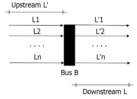
For the simulation model, the structure model is defined following the connections between buses and lines. These connections define a network topology where state events related to lines should be routed. Given a set of n lines L = {L1, L2, …, Ln} entering the bus B, the outgoing lines of B (defined by the set L’) can be considered as located downstream of L. If some event takes place in L (e.g., inactivity), the downstream lines may experience unexpected behaviors (e.g., a transmission line becomes inactive because lines placed upstream have entered fault/maintenance). Figure 1 represents this scheme. Hence, the simulation model outlines the structure of the transmission system using such a scheme, where the foundational component is the behavior of a transmission line (TL). The data produced during the simulation process is recorded in an output file. Such a file contains the state of the TLs along the simulation horizon.

Figure 1 Transmission line scheme. 

On the other hand, the optimization model is structured following the set of buses that define the connections between generators, loads, and TLs. To establish the status of the transmission system, this model uses as input the status of the TLs (obtained from the output file of the simulation model). Based on this data, the model determines the optimal combination of generator units minimizing the production cost function (Frangioni et al., 2009). It also uses the available configuration of the TLs for load dispatch.

Figure 2 depicts how both models are used in our hybrid approach. This diagram presents the relationships between models. The one-line diagram structures both transmission line and generation systems. For the transmission system, the scheduled maintenances are required as input (MaintenanceSchedule.csv). The goal is to use the state of the transmission system (i.e., the simulation output) during the programming of the generation system (i.e., the optimization model output). However, the time unit used in the simulation model (minutes) has more resolution than the one used in the programming (hours). Hence, we use a data transformation process to fit data (from the TL-name.csv files to the TLGlobalState.csv). In this way, the simulation model can execute maintenance and failure events that can take place at any minute of a daily period (i.e., 1440 minutes). Then, the optimization model carries out the schedule of the generation units every 60 minutes (i.e., one hour). Such a period is the most common operation time used for these processes. By following this approach, both models share the data related to the transmission line states.

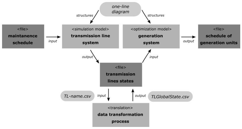
Figure 2 The hybrid structure proposed to link the generation system with the transmission line system through the transmission line states. 

2.2. Transmission System Simulation Model

Figure 3 presents the simulation model using a component-based representation. It is important to denote that, as in any component-based representation, the events that take place as part of the internal behavior of models are not represented. The next sections introduce the behavior of each component.

Figure 3 Structure of the DEVS-based simulation model used to study the transmission system. 

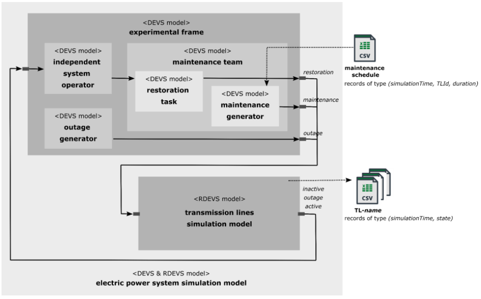
As the figure shows, the overall model is called the electric power system simulation model and is divided into two models (i.e., experimental frame and transmission lines simulation model). The experimental frame is defined as a DEVS coupled model, while the transmission lines simulation model is defined as an RDEVS network model. A DEVS coupled model defines which sub-components belong to a structure and how they relate to each other. On the other hand, the RDEVS formalism has been presented in (^{Blas et al., 2017}) as a subclass of DEVS that provides a solution for the event identification as embedded functionality in simulation models. The core of RDEVS is the abstraction of the event flow as independent behavior of components. Hence, the components to be included in the simulation model can be designed using the DEVS formalism, and then, the RDEVS formalism can be used over them to route events. Given the transmission system topology is defined using the one-line diagram, how components

As the figure shows, the overall model is called the electric power system simulation model and is divided into two models (i.e., experimental frame and transmission lines simulation model). The experimental frame is defined as a DEVS coupled model, while the transmission lines simulation model is defined as an RDEVS network model. A DEVS coupled model defines which sub-components belong to a structure and how they relate to each other. On the other hand, the RDEVS formalism has been presented in (^{Blas et al., 2017}) as a subclass of DEVS that provides a solution for the event identification as embedded functionality in simulation models. The core of RDEVS is the abstraction of the event flow as independent behavior of components. Hence, the components to be included in the simulation model can be designed using the DEVS formalism, and then, the RDEVS formalism can be used over them to route events. Given the transmission system topology is defined using the one-line diagram, how components (i.e., buses and lines) are linked define the routing problem. In this context, the RDEVS formalism provides a suitable foundation for developing the simulation model required at this stage (i.e., the transmission lines simulation model). A RDEVS network model defines the structure of a set of components that are connected all-to-all over a set of routing policies.

All models designed as part of the electric power system simulation model were implemented in Java using DEVSJAVA (^{Arizona Center of Integrative Modeling and Simulation, 2005}).

2.2.2.1. The RDEVS essential ‘transmission line’ model

The formal definition of the essential model that represents a TL is presented in Appendix B. The model starts in an active phase. This means that a TL is initially active. Besides, the model includes two parameters that are used to define the number of inactive upstream lines (parameter named inactiveUpstreamTL, whose initial value is 0) and the total number of upstream lines (parameter named upstreamTL).

In this initial state, the model can receive different events from the experimental frame, namely: maintenance, outage, and restoration. When a maintenance event is received, the model enters a maintenance phase. Before this, the TL warns its downstream lines that it is about to be out of service. To do this, it sends an inactive event. This event is selectively sent only to the lines directly downstream of the current TL. After this sending, the model goes into the maintenance phase for the period defined in the maintenanceTime attribute. When the maintenance is finished, the TL can go into an active or inactive phase (according to the state of the upstream lines at that time). In case of having to enter an active phase, before changing its state, the TL sends an active event to its downstream lines (to inform that from now on, it will be active).

The arrival of an outage event causes the model enters to an outage phase until a restoration event arrives. Because of the outage state, the TL sends an inactive event to its downstream lines (to inform its eventual state of inactivity). Also, it sends an outage event to the independent system operator to manage the repair order. Finally, when a restoration event is received, the model returns to the active or inactive phase (according to the state of the upstream lines). The criteria applied are the same as for the arrival of a maintenance event.

In addition to the events coming from the experimental frame, a TL must deal with the arrival of active and inactive events sent from other upstream TLs. When an active event arrives at a TL, the TL decreases (by one unit) the number of inactive lines upstream (parameter inactiveUpstreamTL). If the line was in an active phase, the model continues as it was doing (because what has happened is that one of the upstream lines has gone from inactive to active). This situation does not affect the current activity of the TL (because there is an active upstream line that allows the TL to remain active). However, if the line was in an inactive phase, the state must change to an active phase. In this case, the model alerts its downstream lines that its entering activity (by sending an active event).

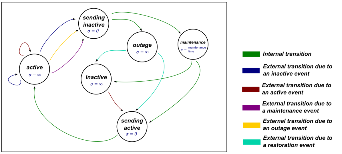
On the other hand, when an inactive event is received in a TL, the model increases (by one unit) the number of inactive lines upstream (parameter inactiveUpstreamTL). If this increase causes that the value of inactiveUpstreamTL to equal upstreamTL, the TL enters an inactive phase (since all upstream lines are inactive). The TL then sends an inactive event to its downstream lines and then goes into an inactive phase. The model will exit this inactive phase when one of its upstream lines informs it that it has entered an active phase (i.e., an active event arrives). On the contrary, if after the increase the values of inactiveUpstreamTL and upstreamTL are different, the TL must remain in an active phase. To provide a more comprehensive definition, Figure 4 presents a state diagram that illustrates the main features of the behavior described before.

Figure 4 State diagram that represents the RDEVS essential model of transmission lines 

2.3. Data transformation process: from simulation output to optimization inputs

As described in Figure 1, the proposed hybrid approach is based on the integration between generation and transmission systems. A data transformation process was developed to achieve such integration. This process allows translating the output data obtained from the simulation model (i.e., related to the transmission system) with the input data required by the optimization model (i.e., the generation system).

The data transformation process analyzes the state of each TL during the simulation time and defines a matrix of TL states for each hour of the scheduling horizon used in the optimization model. The process uses as input information the output files produced by the simulation model (TL-name.csv). These files contain the state of each TL as records of type {simulationTime, state} where the possible states are represented by integer values, namely OUTAGE (0), MAINTENANCE (1), INACTIVE (2), and ACTIVE (3).

Although the simulation model allows specifying several states for the same TL, the optimization model admits only two possible states: ON (1) and OFF (0). Then, to align the state information of both models, our process uses a transformation rule (RT): "A TL in ACTIVE state is equivalent to the ON state, while any other state should be interpreted as OFF state”. Hence, the data transformation process search through all the records of TLs to determine their states in the intervals of the programming horizon (i.e., every hour). The status of each TL is transformed following the RT described. As a result, the transformation process creates a Boolean matrix of global states. Rows are TL and columns represent each hour of the scheduling programming horizon (24 columns to represent daily hour-by-hour scheduling). Such a matrix is stored in a new file called TLGlobalState.csv. As stated before, this file is used as input into the optimization model.

2.4. Generation System Optimization Model

According to (^{International Energy Agency, 2017}), the world energy matrix is composed of the following sources: oil (31.7%), coal (28.1%), natural gas (21.6%), biofuels and waste (9.7%), nuclear (4.9%), hydroelectric (2.5%), and other renewables (2.1%).

As mentioned, the hybrid model employs the proposal presented in (^{Alvarez, 2020c}), which uses the GAMS software and its CPLEX Resolver to solve the optimization problem. That model considers all the mentioned energy sources to schedule electricity generation in Argentina. It minimizes the cost of generating electricity from each of the sources according to (1). This objective function represents the operating cost for producing electricity with all considered technologies. It means the sum of the produced power multiplied by the correspondent cost. The indexes i and t correspond to the unit and the period of the generators. The constants I and T refer to the total number of generators and periods. Besides, the constants δ represent the generation cost per MW, and p is the power output variable. The supra-indexes belong to the different sources: g is the supra-index related to power output for units that work by using natural gas, ng is related to thermal units that work by consuming other fossil fuel different from natural gas, h for hydropower generation, n for nuclear generation, w for wind, and pv for photovoltaic units, respectively. For further details regarding the constraints implemented, they are included in (^{Alvarez, 2020c}).

Demand constraint, described in (2), states that the sum of the produced power of all units must cover the demand, which is composed of the sum of all loads (ld _c,t ). In this equation, ld _c,t is the parameter of load, and c is the correspondent set.

In (3), the spinning reserve is the available power but is not charged, which can compensate for unexpected failures. The equation utilizes a binary variable u _i,t , which is equal to 1 when the generator is operating, and 0 when the generator is shut down. This constraint must be extended to all the considered technologies (natural gas, hydro, nuclear, wind, and photovoltaic).

Generation limits are stated in constraint (4). Where pilo and piup are the lower and upper limits.

Transmission constraints are modeled by using the called DC flow model, which is detailed in (5). This model reaches feasible solutions in addition to a reduction of computational (when the DC flow model is compared with the non-linear models, for instance, the AC model). In this equation, fbui,buo,t is power flow transmitted between the input bus bu _i and the output bus bu _o . Also, Rbui,buo is the reactance of the line.

In (6), the bus balance is performed. The sum of power output, in addition to the entering transmitted flow (fbui=bu,buo,t), is equal to the sum of the leaving transmitted power (-fbui,buo=bu,t), the power storage (SPbu,t), and the sum of loads (ldc,bu,t).

The new model incorporates the transmission of electricity through the lines by using a matrix that represents the current state of each of line. This matrix is directly obtained from the TLGlobalState.csv file. The information in this array is used in (7), where Fline- is the maximum power flow supported by the line (MW), f _line.t is the variable of effective power transmitted, and Γline,t is the array of line state coefficients. Then, the integration between the mathematical models solved in a optimization software and the result of the simulation is performed by creating the matrix Γline,t. In each period, the model uses the updated matrix representing the current state of all transmission lines.

Furthermore, the performance of the model is improved since the processing time is reduced (especially in large-scale systems). This is because the simulation model states that if all upstream lines are offline (i.e., have fallen into inactivity), the next TL will be also offline. This is reflected in the matrix calculation, so the optimization software (at the beginning of the programming period) will not attempt to consider the inactive lines. For this reason, the calculus of possible solutions is reduced. The considered mathematical model offers several benefits in different fields of the optimization topic. First, the model offers representations of different sources that are closer to reality than similar approaches. One example of this statement is presented in (^{Alvarez, 2020b}), where the presented model represents more closely the operating curves by accepting more breakpoints. Another benefit is the reduction of the computational effort due to the implementation of techniques, as the DC power flow model, whose performance, in terms of CPU time reductions, was confirmed in (^{Overbye et al., 2004}). At last, the rest of the benefits of MILP formulation (reduction of computational effort, global optimally, and flexibility to add constraints) were deeply discussed in (^{Lima & Grossmann, 2011}).

Under this scheme, the integration of the simulation results (in addition to the benefits already stated) produces a reduction of the computational effort in the resolution of the optimization model (since the model does not have to evaluate the possibility of power circulation through a previously disabled line. The model presented is a hybrid, a "mixture" of deterministic and stochastic. The presence of a single random variable in the model requires consideration of the model of this nature. Hence, our approach introduces a model that deals with problems characterized by this uniqueness. Given the complexity of the electrical network, along with the action of other elements of the electrical systems, algorithms such as the network simplex algorithm cannot generate appropriate solutions to the system. Due to the complexity of these systems, our proposal is a link between complex electrical systems and their deterministic and stochastic responses.

The saving of computational effort is achieved because the mathematical model presented in this paper combines the implementation of several techniques that were not considered before as an integrated approach. Consequently, the new proposal offers the use of techniques that were previously developed, but they did not consider the totality of aspects that compose an electric system. For instance, some methods improve the computational effort needed to solve the scheduling of a system but, these methods do not consider the existence of all generating technologies (that we are considering in this paper). This paper is composed of detailed mathematical representations that require several methods to improve the CPU times. Besides, these methods must be suited to be applied in the type of problems. The key of this work is not only a collection of approaches but also includes the necessary modifications to be integrated with The RDEVS Essential ‘Transmission Line’ Model.

As it will be observed in the discussion of results (Section 3), the benefits of implementing a MILP model mean a reduction of computational effort. This topic is deeply discussed in (^{Feng et al., 2019}), for thermal and hydro generation. The authors determine that even though a great number of variables and constraints, MILP models achieve satisfactory solutions with reasonable CPU times. Other benefits of MILP approaches in the field of electric power systems are deeply discussed in (^{Koltsaklis et al., 2018}). The performance of the proposed method is tested by considering potential interconnection choices among different systems. Besides, the benefits of solving large-scale problems (in terms of computational effort saving) by considering linearization or reduction techniques are detailed in several papers (^{Alvarez, 2020b}; ^{Lima & Grossmann, 2011}). These papers are not included in the present approach to not overextend the proposal. Besides, the core of this work is not to present advances in the linearization of reduction techniques.

2.5. Case study

Figure 5 shows the one-line diagram that represents the case study. This diagram depicts a system defined as a set of 6 buses, 11 transmission lines, 3 generators, and 3 loads. A detailed description of such a system can be found at (^{Grey & Sekar, 2008}).

Figure 5 6 buses and 11 lines one-line diagram. 

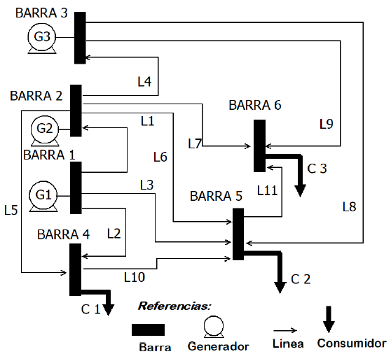
To compare the impact of the use of the simulation model on the optimization model, Section 3.1 presents the results obtained when solving the optimization problem without considering the state of the lines. Then, it shows the results achieved when the hybrid approach is applied. In both cases, the simulation time and the programming horizon are set in one day (1440 minutes for the simulation model and 24 hours for the optimization model). In the case of the optimization model, as previously stated, the solver used by GAMS is CPLEX, and the relative gap is 0.0004 %.

It is important to denote that data of the test system has been extensively studied and proved in the literature. However, these papers do not consider failures in transmission lines. In this regard, as stated before, the utilization of the Weibull distribution has been indicated by many authors as the correct tool to study the random (^{Wang et al., 2016}; ^{Vásquez et al., 2009}). For the scenario where failures should be considered, we propose a specific configuration.

3.1. Electric System without/with transmission line outages

In the first scenario (electric system without transmission line outages), the system described in Section 2.5 is analyzed considering that transmission lines are always available. Following the test case, the optimization model described in Section 2.4 is composed of 2,396 equations, 961 continuous variables, and 336 binary variables. The processing time is 9 seconds, and the total cost is $ 77,423.

Regarding the generation system, the results show that the generator that produces the highest amount of electricity is G1. This generator is operative during the 24 hours, and it generates a total of 5234 MWh. Other generators (i.e., G2 and G3) compensate for the required demand by producing electricity at specific time intervals. Furthermore, the G2 generator is active between 10-17 and 20-23 hours (generating a total of 280 MWh). Besides, the G3 generator produces electricity between 18 and 20 hours with a total generation of 113 MWh. As a result of such a generation process, the lines transmit an electricity flow.

Figure 6 (a) shows the result obtained for these flows. In this case, although all lines are available, there are intervals where some of them do not transmit any electricity. This is because the model optimally changes the flow amount when it reduces the operating costs. For example, the lines directly connected to G1 (which produces the highest amount of electricity) are the ones that have the highest averages of transmitted flow (L2 with 92.5 MW, L1 with 70.4 MW, and L3 with 55.1 MW). These results show that the model minimizes the generation costs by choosing "freely" the most convenient form of transmission over the complete set of lines. For this reason, it is observed that the model always tries to maximize the transported flow through lines connected to the generators with lower production costs.

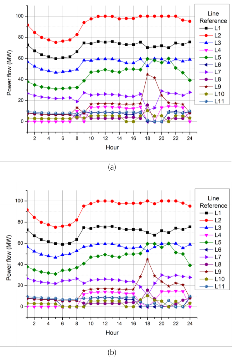
Figure 6 (a) Flow per transmission line in scenario A. (b) Flow per transmission line in scenario B. 

In the second scenario (electric system with transmission line outages), the system detailed in Section 2.5 is studied considering that transmission lines are not available all the time. Hence, the availability of lines is modified by the experience of preventive and unscheduled maintenance events. Then, the parameters of the simulation model are set as follows:

Following this scenario, several simulations were executed. This allows making a deeper analysis of different cases in the optimization model. The number of equations and variables studied in the optimization model remains the same as in the previous situation.

Results indicate that, as more lines are inactive (either by scheduled maintenances or failures), the total cost of production increases. We can observe such an increase is given due to maintenance. Maintenances force generators to produce electricity in a less optimal mode. When there are only scheduled preventive maintenances, the cost increases by 1.2%. However, when unscheduled maintenance is also considered, the cost increases significantly (according to the type and number of lines that are out of service). Costs Vincrease even more when the lines that are out of service are the ones that transmit the generation of cheaper units. This is the case of lines L1, L2, and L3. Such lines transmit electricity generated by G1 (which produces most of the daily generation, as we have described in the first scenario).

In cases where one of these lines becomes inactive due to a failure, the optimization problem cannot be solved. This means that some users cannot be provided. Specifically, this happened when L1, L2, and L3 are out of service simultaneously. Here, the remaining units cannot provide the electricity required to satisfy the scheduled demand. Figure 6 (b) shows the power flows per line for the case where, in addition to scheduled maintenances of L4 and L6, the system has one unscheduled maintenance due to a failure in line L10 between 360 to 599 minutes. In this scenario, besides the periods where lines L4, L6, and L10 do not transmit due to maintenance actions, other periods without transmission are recorded.

In simple examples, this contribution may not seem to have much impact. However, when models that represent large scale systems are solved, this unnecessary calculation causes high processing times that could be avoided. The calculation of power flow through lines implies the determination of angular voltage differences between connected buses if the DC model is used. An example can be observed in Figure 7 (a) where a simulation of 1,440 minutes of the system is performed. It is interesting to mention that the line L11 is still in service all the time, despite the outage of one of its predecessors (L4, L8), because the other predecessors (L6, L3) are still working. In the simulated case, in addition to the scheduled maintenance, an outage of the L9 line is observed, due to a factor external to the scheduled maintenance.

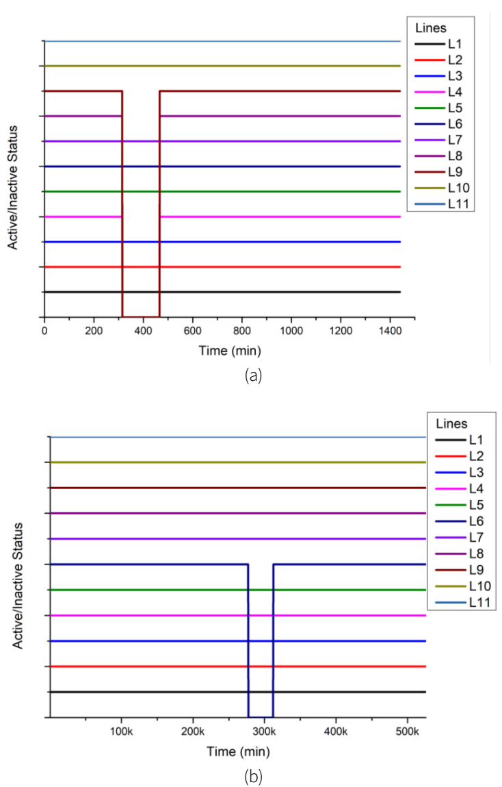
Figure 7 (a) Simulation of 11 lines system for 1,440 minutes. (b) Simulation of 11 lines system for 525,600 minutes. 

In this case, as the line has no successors in the cascade, it does not affect the rest of the lines. More cases have been calculated to study the effectiveness of the proposed approach.

On the other hand, for other simulation case (a simulation for 525,600 minutes, in Figure 7 (b), the line L6 suffers an outage due to an unexpected event, according to the Weibull distribution. It is important to mention that this simulation does not consider scheduled maintenance. This will affect the lines that are in cascade with L6 (L11), although it does not take it out of service because the line receives other feeds that allow it to continue operating. However, disconnected buses must be excluded from the calculation of transmitted power flows.

3.2. Reproducibility in other cases

By studying the results of the test cases proposed in both scenarios, along with the results obtained for other cases available in the literature, the reproducibility of the proposed approach can be studied in detail. Data used in test cases can be found in (^{Alvarez, 2020c}; ^{Badakhshan et al., 2015}; ^{Fu et al., 2005}; ^{Guo, 2012}; ^{Lotfjou et al., 2010}; ^{Norouzi et al., 2014}). The results show the convenience of the proposed models.

For this paper, the models and results obtained in these case studies are detailed to focus the reader's attention on the proposed hybrid approach rather than on the multiple resolutions of the cases.