


 text new page (beta)
 English (pdf)
 Article in xml format
 Article references
 Send this article by e-mail
 Cited by SciELO
  Similars in
SciELO
Similars in
SciELO 
 Permalink
1. Introduction
Researchers often face the need to assess the effect of one or more material’s property after altering its composition and/or manufacturing process (Montgomery, 2001). Additionally, the focus is also on whether the required homogeneity has been achieved in sequential batches, to ensure that the manufacturing process is reproducible. In industrial quality control, for instance, comparisons among samples from different suppliers or even from different manufacturing lots of the same supplier may be needed in order not to add variability to the results either in series production in industry or experimental investigation in laboratory (Duncan, 1986; Juran & Gryna, 1988). Using consistent statistical analysis to evaluate material testing and process variables can improve these desired quality controls.
Analysis of Variance (ANOVA) is a classical statistical test for equality of several population means. Tukey’s test complements the ANOVA by performing all pairwise mean comparisons to identify which mean differs from the other. Both have been jointly applied in materials’ science as by (de Vasconcellos et al., 2006; Felipe et al., 2018; Lee et al., 2020; Moorehead et al., 2018; Rankouhi et al., 2016;), or even other test combinations (Barbosa et al., 2009; Roa et al., 2015; 2016), but almost no works available in the literature mentions if the necessary validation to support their findings has been done.
All statistical tests have a set of model assumptions, that are somewhat violated when the test is applied.
Researchers, in all scientific knowledge areas, poorly exploit robustness analysis and complementary tests requested. Skipping out these steps, the statistical analysis results cannot be trustworthy (Duncan, 1986; Montgomery, 2001). The objective of this work is to fill this gap, presenting a complete statistical analysis of microhardness tests performed on sintered samples of boron carbide.
Boron carbide, in stoichiometric formulae (B4C) is well known as one of the hardest (excluding diamond and boron nitride) and most stable nonmetallic materials. The density of the compound is low (around 2.52 g/cm³), but if others non-pure stoichiometries are considered the density may shift slightly. The high melting point (2450 ºC), Young’s module and hardness provide B4C with outstanding mechanical properties allowing it to the best candidate for severe applications, such as nuclear, medicine and ballistic (Alizadeh et al., 2004; Bouchacourt & Thevenot, 1985; Chen et. al., 2005; Day et al., 2006; Emin & Aselange, 2005; Guo et al., 2019; Hayun et al., 2010; Mortensen et al., 2006; Mondal & Banthia, 2005; Türkez et al., 2019; Vargas-Gonzalez et al., 2010).
Microhardness tests are widely used to characterize mechanical properties of materials, as these tests can provide reliable values of strength limit, yield strength, Young´smodulus, fracture toughness, and hardness value in small volumes of material. This feature enables the evaluation of specific phases or constituent regions or gradients, something incapable of evaluation by macrohardness indentation tests. The microhardness testing consists of quick tests and it allows obtaining a large amount of data over the sample analysis surface. In addition, it requires only a simple flat surface preparation (ASTM E384, 2017).
Although this is a simple test, the microhardness values can be influenced by the indenter's geometry, the applied load, the load application rate, the surface condition of the sample and the microstructure of the material (Lee & Speyer, 2004; Moshtaghioun, 2016; Vargas-Gonzales et al., 2010), especially when it comes to ceramic materials, leading to scattered value (Thevenot, 1991; Ullner et al., 2001). ASTM E384 (2017) microhardness test standard only recommends the calculation of the average and standard deviation, highlighting that microindentation hardness tests will reveal hardness variations that commonly exist within most materials and a single test value may not be representative of the bulk hardness. However, the average and standard deviation do not suffice to conclude if two or more samples are equal or not. Therefore, a deeper statistical analysis is necessary for the interpretation and validation of the results merit.
This paper exposes the serial statistical testing sequence until reaching a solid conclusive analysis on Knoop microhardness tests performed in boron carbide sintered samples, itemizing the critical required heed. It aims at showing the importance of performing a consistent statistical analysis and encouraging material science´s researchers to make use of the well-known statistical tools in their daily life.
The paper is structured as follows: the first part is devoted to descript the boron carbide samples and the microhardness test. The second part encompasses the statistical tests in a logical sequence highlighting their points of attention, discussing and exploiting the partial results before going to the next test, to serve as a route for the reader. The third part discusses the results and presents their agreement with papers published by others.
This paper does not hold experimental uncertainty analysis, the authors recommend the reader to follow standard practices as ISO/IEC Guide 98 (2009).
2. Materials and methods
2.1. Description of samples and Material Characterization
Three dense samples were produced from coarse boron carbide and amorphous boron powders, both supplied by H. C. Starck manufacturer. These powders were mixed in a ratio containing 98.5 wt% B4C and 1.5 wt% amorphous boron (Bam).
The particle size reduction - smaller than 1 micron - was achieved using a planetary ball mill in 200 ml of distilled water at 250 rpm. Milling balls made of SiC, about 350 g, and a steel container with alumina coating were used. Two milling times were set: 30 and 60 minutes (Table 1). The material was dried by evaporation with mechanical stirring at hot plate until it reached a viscosity as slurry and subsequently placed in a heater at 110 °C for 6 hours.
Table 1 Samples’ milling time, press load, post-sintering densification, porosity and densities.
| Parameters | Samples | ||
|---|---|---|---|
| A | B | C | |
| Milling Time [min] | 60 | 60 | 30 |
| Press load [N] | 9800 | 4900 | 4900 |
| Theorical density [g/cm³] | 2.52 | ||
| Archimedes' apparent density [g/cm³] | 2.44 | 2.43 | 2.34 |
| Apparent porosity [%] | 5.02 | 4.17 | 12.73 |
| Post sintering densification [%] | 96.83 | 96.43 | 92.86 |
| Rietveld density [g/cm³] | 2.57 | 2.61 | 2.70 |
| Relative densification [%] | 94.94 | 93.10 | 86.67 |
To the dry material were added 1.0 wt% of polyvinyl alcohol (PVA, Vetec brand), 1.0 wt% polyethylene glycol (PEG, Oxiteno brand) and a drop of defoamer. It was homogenized for 8 hours in a planetary ball mill at 250 rpm and then dried at 110 °C for 6 hours.
The content was manually macerated for deagglomeration and sieved in vibrating sieves of 0.84 mm, 0.42 mm and 0.25 mm. To understand a possible influence of the milling time on the green density and sintered density, the material was compacted by uniaxial pressing (Carver hydraulic press mod C) under pressures of 4900 N for samples A and C and 9800 N for sample B (Table 1). A tempered steel mold of 15 mm was used for that.
After uniaxial pressing, the pressed green bodies were vacuum encapsulated in a latex matrix and isostatically cold pressed in an ABB Autoclave Systems isostatic press, model CIP62330, under the pressure of 150 MPa (about 22 kpsi). Sintering was performed in a Series 45 Top Loaded Vacuum Furnaces furnace, model 45-6x9-G-G-D6A3-A-25 (Centorr Vacuum Industries), with the green bodies wrapped in graphite sheets. Low pressure sintering was conducted at a heating rate of 10 ºC/min to 1,800 ºC, isothermal of 30 min and cooling the oven at a controlled rate of 10 ºC/min, as reported by Couto et al. (2012). The values of post-sintering densification, apparent porosity and relative density are presented in Table 1.
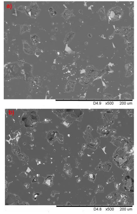
The milling powders passed through a Cilas 1064 laser particle size analyzer. One mg of each sample was diluted in a ratio of 2 ml of sodium hexametaphosphate to 10 ml of distilled water. The particle size distribution d10, d50, and d90 was 0.07, 0.28, and 2.20 μm, respectively, showing that a lower limit particle size was achieved for the comminution processed used, independent of the milling time. Contaminant elements were identified in samples by energy dispersive spectroscopy (EDS) and X-ray diffraction (XRD), as well as analyzed and quantified by the Rietveld method. Although it is not the main scope of this work, some data will be presented to illustrate the results. It was used a PANalytical X’PERT PRO diffractometer, with Cu-Kα radiation, 2θ varying 10º to 100º, step of 0.05º and 30 s per step. Microscopy images were obtained using a Hitachi TM 1000 model scanning electron microscopy (SEM) equipment, with an energy dispersion microanalysis system (EDS) model Link Isis L 300 with 15 kV acceleration of the electron beam. Figure 1 shows micrographs of samples B and C, as examples of post-sintered microstructures. It is possible to observe that the milling time directly influenced the presence of defects (porosity) of the material. The lightest areas refer to the SiC phase.
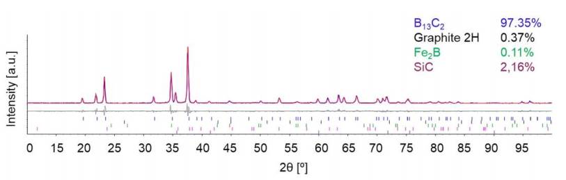
These contaminants are possibly coming from the milling accessories, such as SiC balls and WC from the container liner. The found elements were Si, Fe, Cu, Al, W, being identified the phases C(2H), SiC, WB2.5 and Fe2B, besides B13C2 - expected stoichiometry for Boron Carbide - as described in Table 2. Figure 2 shows the XRD pattern for C sample as an example of the analysis. The refinement was made using TOPAS Academic v.4.1. The blue curve indicates the experimental data and the red one the calculated data. One can see a good signal-to-noise relation in the experimental data that improved the goodness of fit (GOF) of the Rietveld calculations, which was 1.68. As it can be noticed, this difference was tiny, leading to a lower deviation in the phase quantification.
Table 2 Samples’ phase content obtained by XRD refinement.
| Phase | Samples | ||
|---|---|---|---|
| A | B | C | |
| B13C2 | 96.40% | 96.47% | 97.35% |
| C(2H) | < 1% | < 1% | < 1% |
| Fe2B | < 1% | < 1% | < 1% |
| WB2.5 | < 1% | < 1% | < 1% |
| SiC | 2.60% | 2.18% | 2.16% |
It is verified that the densification increased as the milling time also increased. High energy milling usually comes along with sample contamination. In fact, high energy milling processes lead to particle size reduction, higher surface area and higher degree of contamination as comminution time increases.
Regarding contamination, the SiC came from the milling balls, having the same quantity for all milling time. XRD semi-quantitative analysis has revealed a contamination level lower than 1%, indicating C, WB2.5 and Fe2B phases. Sample C had slightly lower contamination than samples A and B. Higher concentrations of Fe2B, C(2H) and WB2.5 in A and B in relation to C indicate that these phases favored the process of densification of the samples during sintering (Chen et. al., 2005; Zakhariev & Radev, 1988).
The Rietveld (crystallographic) density found was higher than the theoretical density of the material, perhaps due to the presence of closed pores. The relative densification was calculated considering the relative percentage between the Archimedes’ (ABNT NBR 16661, 2017) and Rietveld densities. The Rietveld method assesses the phase density over the entire sample volume, while the Archimedes’ method is sensitive to the presence of superficial, interconnected and closed pores in the sample.
2.2. Knoop Microhardness Test
The Knoop microhardness measurements were conducted in the Panambra Microdurometer, model HXD-1000TM brand Pantec, equipped with an optical microscope up to 600x magnification and digital camera with a resolution of 1.6 Mpixels for image capture. It was used a Knoop indenter (diamond pyramid).
Twelve valid indentations were performed in each sample, randomly distributed, with a fixed load of 500 g for 15 s, at a temperature around 25 ºC. Indentations according to ASTM E384 (2017) and ASTM C1326 (2008) were considered valid. For this, the surface of the sintered samples was abraded at #200, #400, and #600 and polished at 1 µm diamond paste.
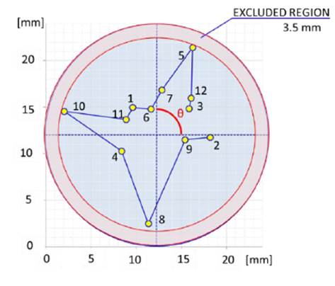
In order to guarantee the randomness of the points measured and the homogeneity for all samples, an automatic sampling generation system was established during the hardness test. The location of each measure is given by the ordered pair constant, being a radial distance (x, y) and an angular measure (θ) in relation to the sample center, uniformly distributed, unbiased and delimited by the radius of the ceramic piece, excluding the edge region, as shown in Figure 3.
3. Results and Discussion
3.1. Knoop Microhardness Test
The results of the Knoop microhardness measurements in each indentation are presented in Tables 3, 4, 5 for samples A, B, and C, respectively.
Table 3 Knoop hardness in each indentation of A sample.
| A | |||
|---|---|---|---|
| Indentation # | Knoop hardness (HK) | Indentation # | Knoop hardness (HK) |
| 1 | 2,254.0 | 7 | 1,972.9 |
| 2 | 2,240.6 | 8 | 2,439.7 |
| 3 | 2,490.3 | 9 | 2,326.3 |
| 4 | 2,159.2 | 10 | 2,497.0 |
| 5 | 2,248.0 | 11 | 2,284.8 |
| 6 | 2,268.5 | 12 | 2,218.0 |
| Mean | 2,283.3 | ||
| Standard deviation | 146.2 | ||
Table 4 Knoop hardness in each indentation of B sample.
| B | |||
|---|---|---|---|
| Indentation # | Knoop hardness (HK) | Indentation # | Knoop hardness (HK) |
| 1 | 2,303.6 | 7 | 2,564.0 |
| 2 | 2,414.1 | 8 | 2,384.9 |
| 3 | 2,353.9 | 9 | 2,240.6 |
| 4 | 2,339.1 | 10 | 1,916.6 |
| 5 | 2,326.3 | 11 | 2,386.4 |
| 6 | 1,879.7 | 12 | 2,284.8 |
| Mean | 2,282.8 | ||
| Standard deviation | 196.9 | ||
Table 5 Knoop hardness in each indentation of C sample.
| C | |||
|---|---|---|---|
| Indentation # | Knoop hardness (HK) | Indentation # | Knoop hardness (HK) |
| 1 | 1,979.5 | 7 | 1,944.5 |
| 2 | 1,968.0 | 8 | 2,220.7 |
| 3 | 1,989.5 | 9 | 2,019.5 |
| 4 | 1,986.9 | 10 | 2,307.7 |
| 5 | 2,062.9 | 11 | 2,117.1 |
| 6 | 1,962.2 | 12 | 2,189.6 |
| Mean | 2,062.34 | ||
| Standard deviation | 119.5 | ||
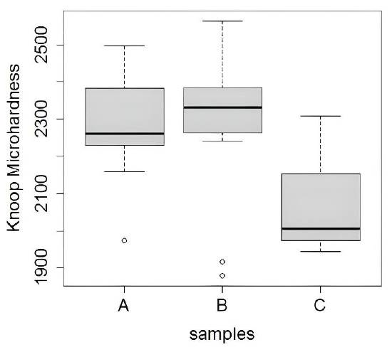
Figure 4 shows a boxplot of Knoop microhardness values.
3.2. Statistical analysis
Section 2.2. showed that samples A, B and C have different chemical and structural composition which could influence their microhardness. On the other hand, section 3.1 presented very close measured Knoop microhardness between samples A and B, and an only 8% less value for sample C. Then, the interest in knowing if samples A, B and C have or not the same hardness arises.
This section aims at describing the full procedure followed in the post hoc statistical analysis of the Knoop microhardness tests to reach an accurately assured conclusion.
3.2.1. Data consistency
A first stage of any analysis should be exploring the data (Kozac & Piepho, 2017).
Before starting the analysis of variances (ANOVA), all data must be checked about their consistency. Outlier searching is an essential step.
An outlier is an observation point that is far from the others. An outlier may be due to variability in the measurement or it may indicate an experimental error; in the latter case, this observation must be excluded from the dataset. To eliminate outliers is mandatory, although this could generate unbalanced data, i.e., unequal sample sizes. The power of the test is maximized if the samples are of equal size (Montgomery, 2001).
All data have passed through the Z-score test for outliers checking. The maximum absolute value found was 2.12, so there is no outlier in this analysis. Data processing was performed separately for each group.
Sorting the order of execution is required to assure that all indentations are independent. After, in residual analysis, residuals must be found independent of the order of execution.
The independence of the observations is one of the most important ANOVA assumptions (Kozac & Piepho, 2017).
The used Knoop equipment has a polar coordinate system, so it is easy to follow the shortest path always searching for the next closest sampling point. Additionally, it is more convenient to execute sequentially all indentations on the same sample before starting testing the next sample.
If so, a critical model assumption for ANOVA has been violated, that all observations are mutually independent. Only if residuals are confirmed to be normally and independently distributed (NID) with zero mean and residuals are independent of the execution order, the results from the ANOVA analysis can be used.
3.2.2. Checking one ANOVA model assumption before performing the analysis
One ANOVA assumption is the equality of variances. A widely used procedure is the Bartlett test (Montgomery, 2001) for multiple comparisons of sample variances.
Since the Bartlett’s test is sensitive to the normality assumption, a modified Levene’s test is more useful, because it is more robust in relation to departures from the normality.
To test the equality of variances among all treatment means, the modified Levene’s test uses the absolute deviations of the observations in each treatment from the treatment median. The test’s statistic for the Levene’s test is simply the usual ANOVA F statistic for testing equality of means applied to absolute deviations (Montgomery, 2001).
Table 6 shows the ANOVA table corresponds to the results from the modified Levene’s test for equality of variances of microhardness tests from samples A, B, and C. There is no evidence for rejecting the hypothesis of equality of variances, after comparing the calculated p-value with the prefixed significance level at 0.05. The p-value is the smallest level of significance that would lead to rejection of the null hypothesis (Montgomery, 2001). DF represents Degrees of freedom and MS is means square.
3.2.3. Analysis of Variance (ANOVA)
Analysis of Variance (ANOVA) is an extension for comparisons among several population means, of the classical t-test for comparison between two population means.
The null hypothesis assumes that all means are equal. The alternative hypothesis states that at least one mean differs from the others. All tests of hypothesis are conceived for rejecting the null hypothesis. There is some misunderstanding that not rejecting the null hypothesis could be the same of accepting it, in this case the correct statement is that there is no statistical evidence to reject the null hypothesis at the significance level selected. ANOVA, as others statistical hypothesis tests, limits the probability of type I errors to a prefixed significance level and controls the probability of type II errors by choosing a suitable sample size taking into account economic and time limitations.
This study is focused on the response in Knoop microhardness from 3 different material samples that correspond to 3 treatments (or levels) of a unique factor.
So, this investigation is defined as a one-way ANOVA because there is a unique factor under analysis, the material samples. The model is of fixed effects because the 3 specimens under test are fixed. Therefore, any conclusions from this analysis are valid only for comparisons among these 3 material samples tested. This analysis is referred to as balanced because all samples have equal size. The 36 microhardness measurements are named observations and their differences in relation to each corresponding sample microhardness mean are residuals, in this case. Table 7 shows the results from the one-way ANOVA, model of fixed effects. DF represents Degrees of freedom and MS is means square.
Table 7 One-way ANOVA, model of fixed effects.
| Source of variat. | Sum of squares | DF | MS | F0 | p- value |
|---|---|---|---|---|---|
| Between treat. | 389,787 | 2 | 194,893 | 7.858 | 0.00162 |
| Errors | 818,472 | 33 | 24,802 | ||
| Total | 1,208,26 | 35 |
The null hypothesis is rejected due the test statistic F0 at 7.858 is greater than its critical value of 3.2849 at the selected 5% significance level for the Fisher-Snedecor probability function with 2 degrees of freedom for the numerator and 33 degrees of freedom for the denominator. The same conclusion is reached by noting that the calculated p-value 0.00162 is less than the significance level. Therefore, there is a difference for at least one microhardness means among samples A, B, and C, but this statement is trustworthy only if the validity of the ANOVA model is proven.
3.2.4. ANOVA´s model adequacy checking
Decomposing variability in observations through an analysis of variances to formally test for no differences in treatment means requires that certain assumptions are satisfied: the model adequately describes the observations and the errors are normally and independently distributed with mean zero and constant but unknown variance. The model adequacy checking is performed through the examination of residuals. If this step is jumped, nobody can rely on its results.
Kozac & Piepho (2017) explain why the normality assumption must be checked in residuals and not in the raw data, and defends that both normality and homogeneity of variance must be checked through diagnostic plots rather than using significance tests. The actual assumption is that the dependent variable should be normal within each group (treatment). This assumption is equivalent to the assumption of normality of errors from the linear model on which ANOVA is based. The errors cannot be directly observed, but are estimated from residuals. Checking residuals will be more powerful because of a greater sample size comparing to checking the observed data within each group.
Generally, standardized or studentized residuals are better for checking assumptions than raw residuals, because the latter may exhibit heterogeneous variance even when errors have constant variance, although for the special case of a balanced one-way both are equally adequate (Kozac & Piepho, 2017).
3.2.4.1. Normality assumption
An extremely useful procedure is to construct a normal probability plot of residuals (Montgomery, 2001), as normal quantile-quantile plot (Q-Q plot) shown in Figure 5. Even though the graphical methods can serve as a useful tool in checking normality for the sample of n independent observations, they are still not sufficient to provide conclusive evidence that the normal assumption holds (Razali & Wah, 2011). There are several formal tests about the normality of sample data, Table 8 presents a set of them, with their results, generated by the R-software (R Development Core Team, 2009). The normality of residuals was not rejected at 0.05 significance level in all tests. Razali and Wah (2011), among others, concluded that Shapiro-Wilk test is the most powerful normality test, becoming recognized as enough for normality assumption checking.
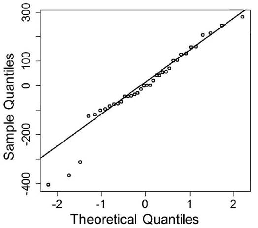
Table 8 Results of normality tests.
| Test | Test's statistics | p-value |
|---|---|---|
| Kolmogorov-Smirnov | D = 0.12524 | p = 0.1635 |
| Cramér-von Mises | W2 = 0.0772 | p = 0.2185 |
| Anderson-Darling | A2 = 0.60312 | p = 0.1086 |
| Lilliefors | D = 0.1252 | p = 0.1635 |
| Shapiro-Wilk | W = 0.94516 | p = 0.0737 |
The hypothesis test is formulated to reject the null hypothesis, that data are sampled from a Normal population. But not rejecting the null hypothesis does not assure that data are from a Normal population. High departure from Normal distribution of residuals can cause serious problems to the ANOVA.
In general, moderate departure from normality is of little concern in the fixed effects analysis of variances. The analysis of variances is robust to the normality assumption (Montgomery, 2001).
The presence of one or more outliers in residuals can seriously distort the analysis of variances.
All residuals have passed through the Z-score test for outlier checking. The maximum absolute value found was 2.64, so there is no outlier in residuals.
A rough check for outliers is usually made by examining the standardized residuals (ASTM C1326, 2008). This is made dividing each residual value by the mean square of the errors. The maximum absolute value found was 2.67.
3.2.4.2. Plot of residuals in time sequence
Figure 6 shows the plot of residuals in time sequence. There is no observation of trends.
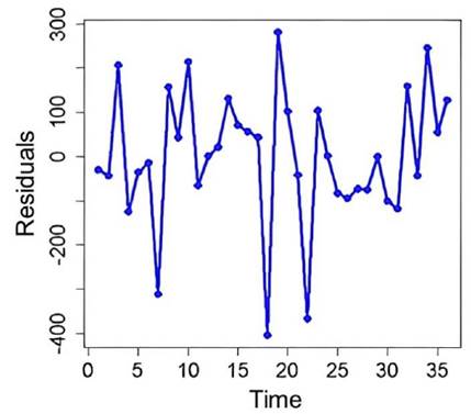
Some criteria proposed by Nelson (1984) for searching indications of no randomness in Control Charts in statistical control of processes were additionally verified: nine successive points below or above the mean, six successive points rising or decreasing and fourteen successive alternating points. None of them is present in Figure 6.
If any hysteresis error is present, this can be viewed at this step. A practical example is a progressive wear of the indenter during test executions. Sorting the execution order can distribute this effect through all specimens under test, smoothing it. This is an example of a systematic error; firstly, it must be avoided, for example, by microscopic inspection of the indenter before starting each measurement. If this cannot be done, and this wear has a deterministic behavior, the measurement results ought to be corrected by eliminating this and any other known systematic error.
3.2.4.3. Plot of residuals versus fitted values
Residuals should be unrelated to any other variable, including the predicted response. For the one-way ANOVA, the predicted values are the means of each group, microhardness means from samples A, B, and C in this case. Figure 7 shows the plot of residuals versus fitted values.
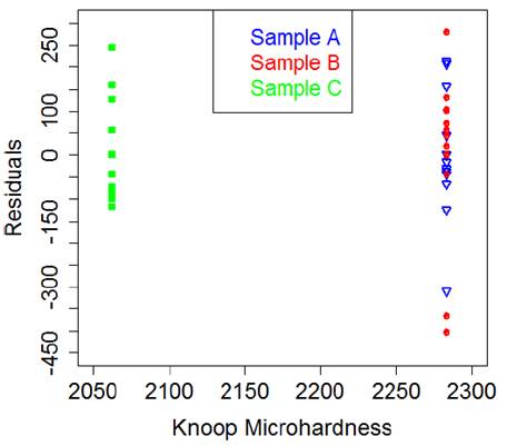
This plot highlighted a difference in variances among the groups, but the data has passed through the modified Levene’s tests as exposed in section3.2.2.
If the assumption of homogeneity of variances is violated, the F-test (ANOVA) is only slightly affected in the balanced fixed effects model (Montgomery, 2001).
3.2.4.4. Plot of residuals versus other variables
There was not identified any other variable that could influence the results. If the experiments were executed in ambient without temperature and humidity control, it was required to plot residuals versus environmental variables, to assure that they have not affected the test results.
3.2.5. Tukey’s test
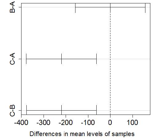
ANOVA’s results have shown that there is a difference for at least one of the three treatment means. But it is of interest of the research to know which(s) mean (s) differ from the other(s). Tukey’s Honest Significant Difference test is suited to test all pairwise mean comparisons.
For equal sample sizes, Tukey’s test declares two means significantly different if the absolute value of their sample differences exceeds the test critical value.
Multiple comparison through a Tukey’s test revealed that there is significant difference between group C from both A and B, that have been shown to be similar (Table 9). The p-value after adjustment for multiple comparisons was 1 to A-B and 0 for both A-C and B-C.
Table 9 Results of the Tukey’s test.
| Paired comparison | Differences | p-value adjusted |
|---|---|---|
| A - B | 0.400 | 0.9999787 |
| A - C | 220,933 | 0.0044756 |
| B - C | 220,533 | 0.0045501 |
Figure 8 shows the 95% family-wise confidence intervals for all pairwise difference in means among samples A, B and C.
3.2.6. Comparison between sample means of A and B grouped with C
Since in the previous section it was found that samples A and B seem to have the same microhardness, a data rearrangement may be done.
According to section 2.1, specimens A and B are distinct since their fabrication processes. However, the t-test for comparison between means from A and B resulted in a p-value of 0.995543. From the statistical perspective, they have the same microhardness, although they have distinct chemical composition and density, as shown in Tables 1 and 2. Anyone would state that samples A and B have come from the same material in the lack of information about their origins and without additional characterization tests. Referring only to the microhardness, it is possible to group A and B and apply a single t-test for comparison between two means, those from A and B grouped against C. However, it was necessary to previously test if A and B have the same variance before assuming that data A and B have come from the same population of microhardness values.
The classical F-test for equality of variances resulted in a p-value of 0.227377. Therefore, there is no evidence for rejecting the null hypothesis based on data available at 5% significance level.
The above-proposed t-test resulted in a p-value of 0.000302, so it is secure to state that specimen C has a different microhardness.
It is possible to construct a 95% confidence interval for the difference between these microhardness means, based on the t-distribution. The lower and upper limits of this interval is 111.5 and 332.2, respectively. Based on this analysis, in other words, the microhardness of sample C is at least 111.5 and no more than 332.2, inferior to the microhardness of samples A and B. After reaching an assured conclusion, the discussion now is about what could have justified the equality of microhardness between samples A and B, and the difference from them in relation to sample C.
Adding more statistical analysis, the microhardness presented greater correlation with phases WB2.5 and C(2H) (Radev & Zakhariev, 1998) and apparent density and post-sintering densification, expressed by the respective Pearson’s correlation coefficients of 0.9998, 0.8893, 0.9974, and 0.9939, as shown in Table 10. Likewise, Pearson's correlation coefficient of 0.5506 for SiC is shown, reaffirming that the phase has little influence on the microhardness of the samples.
4. Conclusions
Control failure during manufacturing randomly produced different level of presence of contaminants in the three boron carbide samples. Although all have different compositions, the post hoc statistical analysis through traditional ANOVA and Tukeys’ test concluded that samples A and B do in fact have the same microhardness, which differs from that of C. For taking advantage from this fortuitous fact to support investigating the effects of contaminants on the microhardness of these samples, a high degree of confidence in this statement was reached, after performing a complete statistical analysis.
It is well known that, in bulk configuration, mechanical properties of sintered ceramics depend strongly on porosity, contaminant phases, grain boundaries characteristic’s and much on point, linear or volumetric defects. Considering the chemical and structure composition of samples, Si, Ca, Fe, Cu, Al, Cr and W contamination verified by EDS and confirmed by phase identification by XRD, microhardness was strongly influenced by the contaminant phases. C sample presents lower presence of SiC, Fe2B and C(2H) than A and B samples besides not presenting WB2.5, therefore, the sample with the least microhardness values since it is well known the influence of additional phases, mainly borides (Couto et al., 2012; Ma et al., 2017). Other important characteristic of the samples to consider is its porosity. By results, the C sample lower microhardness values are associated with C sample porosity (12.73%), while A and B sample porosity is similar (5.02% and 4.17%, respectively). In other words, sample porosity is A ≈ B < C, and the inverse happens with microhardness values, A ≈ B > C.
Nanomechanical behavior of the hydrated nanocomposites concrete, bone and shale is governed by packing density distributions of elementary particles delimiting macroscopic diversity (Ulm et al., 2007). That said, the conclusion is that the post-sintering, influenced by contaminant phases has dictated the microhardness measurement results in this study case.

