


 text new page (beta)
 English (pdf)
 Article in xml format
 Article references
 Send this article by e-mail
 Cited by SciELO
  Similars in
SciELO
Similars in
SciELO 
 Permalink
1. Introduction
Nowadays, navigation systems are involved in many applications in different life-fields. This leads researchers to investigate the development of navigational techniques to reduce the navigation estimation errors and achieve the best results with lowest prices. Therefore, the development of navigation systems using MEMS inertial sensors is taken into account with the navigation system industry. MEMS inertial measuring units (IMUs) are characterized by low-cost and light weight. Development of MEMS based INS is usually difficult due to its high error rate and high deviation of the readings over time (EIdesoky, Kamel, Elhabiby, & Elhennawy 2017a; Hazry & Zul, 2009; Maklouf, Ghila, Abdulla, & Yousef, 2013). GPS receivers provide more accurate and continuous positioning, but with a lower measurements rate. Furthermore, satellite signals are not always available in different conditions such as urban canyons, tunnels, and even indoor situations such as parking garages. Although GPS/INS integration has proven to be a reliable solution (Aftatah, Lahrech, Abounada, & Soulhi, 2016; Shin, 2005) still there are problems when GPS signals are not available. Generally, to overcome this problem, data collected from different additional navigational sensors are acquired, fused and processed to increase the navigation accuracy and we refer to this kind of fusion by MSDF. Currently, the trend is how to overcome the dependence on the GPS by increasing the number of sensors used in navigation; therefore recently, all sources positioning navigation (ASPN) is a very important branch for many researchers in the field of navigation to achieve low-cost, robust, accurate and effective navigation solutions, whatever the availability of GPS (Penn, 2012).In addition, the design of integrated system using a good estimator is an important as same as the significance of increasing the number of navigation sensors to have more reliable, accurate and robust navigation system. All the inertial sensors, microcontroller boards and processor boards which are used in our land vehicle navigation application have been chosen based on the cheapest hardware in the market with an extremely low-performance to be as a challenge to verify the proposed algorithm, a continuous localization solution with a very good level of accuracy performance has been achieved based on our proposed algorithm. A lot of researchers did outstanding efforts toward the objective of this work. To name a few, Xu et al. proposed a reliable hybrid positioning methodology for ground vehicles based on MEMS sensors and approximately costs 4500 ($) (Xu, Li, Li, Song, & Cai, 2016). Zhang et al. proposed a 500$ forward velocity model that depends on the non-holonomic constraints and has been tested by STIM300 IMU from Sensonor (Zhang & Niu, 2018). Nevertheless, other researchers have started to pay attention to another low-cost and grade inertial sensor such as the work proposed by Ahmed and Tahir (2017), via utilizing the measurements from L3GD20 IMU by ST Microelectronics which approximately cost 10 ($) to evaluate a vehicle attitude estimation. The proposed system presented in this work is based on the extremely low-cost and grade inertial sensors MPU-6050 IMU from InvenSenseTM. The achieved real time land vehicle localization solution approximately costs 7 ($) per unit. This IMU and its series can be easily found in various electronic stores or in e-marketing applications. What's more, it is widely used in the field of control systems for robots or small unmanned systems due to light weight, low-cost and low-power consumption. In this work, the additional sensors which we used are the odometer and the magnetic compass. The proposed loosely coupled integrated GPS/INS/odometer/magnetometer system provides an increasing of the accuracy and robustness of the navigation solution and enhanced the positioning estimation unlike using a separate GPS or standalone INS system. The common solution algorithm for GPS/INS integration is the Extended Kalman Filter (EKF). However, EKF depends on the basic assumptions linearization of the nonlinear system and Gaussian noise distribution (El-Sheimy & Youssef, 2020), and the INS 1st order linearized error model is usually used. Although this assumption has proved to have a very good performance, it still associated with low-cost MEMS sensors but in the case of weak GPS signals, noisy environment or outage signals, the performance is degraded. Unlike the EKF, the unscented Kalman filter (UKF) doesn’t require a linearized model and directly it can be applied to the nonlinear model and it is easier to implement because it doesn’t need analytic derivation or Jacobians as the EKF (Julier & Uhlmann, 1997; Van der Merwe, Wan, & Julier, 2004), The usage of UKF for navigation sensors data fusion is discussed in detail in the context of this paper. For further improvement of attitude angles, the complementary filter (CF) has been used to fuse the estimated angles from both the gyroscopes and accelerometers that construct the IMU. CF applies a low-pass filter to accelerometer measurements and a high pass filter to the integrated gyroscopes measurements to improve the attitude estimation. The objective of this work is to evaluate and validate the performance of the position estimation, by implementing a low-cost integrated navigation system based on a selected extremely low-cost and grade MPU-6050, that consists of three-axis accelerometers, three-axis gyroscopes and three-axis digital compass. Three microcontroller boards are interfaced together, two platforms of 32-bit ARM core microcontroller boards with 512 KB memory (one of them is used to perform navigation arithmetic calculations of the inertial sensors and the other is used to process a low-cost commercial GPS receiver). The third platform is a 16-bit AVR ATMEL microcontroller board which connected through CAN BUS with OBD shield to acquire the ground speed measurements. Signal acquisition, mechanization modeling, CF and UKF processes are performed via three boards for real-time calculations. IMU, odometer and GPS raw measurements data are also logged for further post processing under MATLAB for system tuning and offline integration evaluation which helps in the enhancement of the system performance.
In the next sections, the sensors models are presented in section (2), section (3) describes the CF and UKF filters theories, section (4) presents a loosely coupled GPS/INS/Odometer/Magnetometer system implementation by utilizing UKF, section (5) shows the evaluation of the experimental work and results. Finally, the conclusion is presented in section (6).
2. Sensors Modeling
2.1. INS sensor model
The INS mechanization equations are used to obtain the navigation solutions position, velocity, and attitude (PVA) of the vehicle in the East-North-Up (ENU) navigation frame (n-frame), which is known as local-level frame (LLF). These solutions are derived from the angular rates measurements acquired from the three gyroscopes and specific forces measured from three accelerometers as shown in Figure 1. (Aggarwal, El-Sheimy, & Noureldin, 2010).

The acceleration is measured by the accelerometers in the body frame, and then transformed to the navigation frame for getting useful information. This operation is done using the transformation matrix through the attitude angles that are obtained from integrating the gyro rates. The projected acceleration is purified from Coriolis motion and the external effects of gravity by getting pure implication of the body motion. The output is integrated to obtain position and velocity as described in (Noureldin, Karamat, & Georgy, 2012).
2.2. Odometer sensor model
The odometer is a self-independent sensor which measures the land vehicle travelled distance over time, and it is used for continuously estimating the ground vehicle speed without any external interference to improve the navigation performance; especially during GPS outages. With the assumptions of the non-holonomic constraints which is the vehicle does not jump-off or slides on the ground, the vehicle velocity in the plane perpendicular to the forward direction is almost zero (Sukkarieh,1999). These constraints can be considered as a zero velocity update (ZUPT) along two axes of the vehicle (up and right).
where
2.3. Magnetometer sensor model
Magnetometer measures the earth's magnetic fields in its three axes X, Y and Z, so the heading can be determined in the horizontal planes, X and Y. The magnetometer measurements must be compensated for the effects of nearby ferrous materials by calculating the bias and offset in a process called hard-iron and soft-iron compensation. Once the measurements are corrected, the declination angle is applied to adjust magnetic north to true north.
A simple calibration method can be used to determine the offset and scale factor values, by mounting the compass in the car and taking a circular path on a horizontal surface, then getting the maximum and minimum values of the X and Y magnetic readings as follow:
where,
Heading=Heading + declination angle
The used declination angle
3. Complementary and Unscented Filters
3.1. Complementary Filter
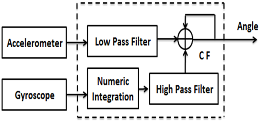
For more precise orientation estimation, accelerometers and gyroscopes are used together. The gyroscope data is useful in a short-time term because the integrated angle from the gyroscope drifts over time; while, the accelerometer data is useful in the long-time term because the accelerometer has a slow response calculation time for calculated tilt angles. The complementary filter is designed in such a way that the strength of one sensor will be used to overcome the weaknesses of the other sensor which makes each complementary to the other. The algorithm is given by:
where:
The tilt angle by accelerometer is calculated by measuring the gravity component in the horizontal accelerometers, then the estimated pitch and roll angles can be calculated. The CF combines the high-pass filter estimations from integrated gyro measurements with the current angle value and low-pass filter estimations from accelerometers measurements as shown in Figure 2. The CF algorithm is applicable in the conditions of low-body accelerations or nearly constant vehicle velocity which is the case of the designed experiments. For higher acceleration conditions such as racing cars or maneuvering missiles, this algorithm is no longer valid due to high dynamic motions.
3.2. Filter coefficient calculation
The time constant
3.3. Unscented Kalman Filter
The system state distribution and its relevant noise densities with respect to EKF are approximated by the Gaussian random variable (GRV), which are propagated analytically through a first-order linearization of the nonlinear system. Hence, the methodology of EKF can be introducing large linearization errors in the true posterior mean and covariance of the GRV transformation, which may lead to suboptimal performance. The UKF can be overcome the linearization errors problem by using a deterministic sampling approach. By using this approach, the system state distribution can be approximated by a GRV which represented by using a minimal set of carefully chosen weighted sample points. These sample points completely capture the true mean and covariance of the GRV, and then propagate through the true nonlinear system, then capturing the posterior mean and covariance accurately to the 2nd order Taylor series expansion for any nonlinearity.
3.4. Unscented Transformation
The unscented transformation (UT) is a technique for determining the statistics of random variable that has a nonlinear transformation. Consider propagation a random variable x (dimension L) through a nonlinear function
Where,
The mean and covariance for
with weights
where
Figure 3 gives an example for a two-dimensional system, Figure 3a shows the Monte Carlo sampling true mean and covariance propagation, Figure 3b represents the output by linearization approach as the EKF and Figure 3c shows the performance of the UT for five sigma points.

Figure 3 Example of the UT for mean and covariance propagation: (a) actual; (b) first- order linearization (EKF); (c) UT. (Wan, Van Der Merwe, & Haykin, 2001).
3.5. Unscented Kalman filter Implementation
The UKF can be implemented using UT method by expanding the state space to include the noise component
Initialization parameters:
where
1. t = k-1
2. Sigma Points
Where
3. The time update equations are:
Propagation of the sigma points through the system equation
The augmented sigma points is
4. Filtering
Where

3.6. Observation
After the observation information collected from the aiding inertial sensors, the observation vector can be generated as follow. In case of GPS is available then the position and velocity observation will be obtained from GPS receiver while, the heading observation angle will be obtained from magnetometer and the measurement vector will be as follow
The observation model is
where
The observation noise covariance matrix is
where
where
The observation vector will be
The observation model is
The odometer observation noise covariance matrix for x, y and z axes in b-frame is
While the odometer velocity is transformed from the body frame to the navigation frame; as well its related observation noise covariance matrix has to be transformed, this transformation is done by
The observation noise covariance matrix is
3.7. Loosely coupled GPS/INS integration
In this integration type, the GPS and INS operate independently and each one provides separate navigation information but the GPS signal information used to aid the INS mechanization to reduce the INS errors which increase rapidly with time and this aiding can be done by GPS measurement update via the step of integration filtering. Furthermore, the navigation solution performance will be improved after the estimated error states feeding to the INS mechanization. Frequently, this integration is based on Kalman filtering as shown in Figure 5, here we have implemented the proposed integration technique based on the unscented Kalman filter (Hieu & Nguyen, 2012).

4. Integrated System Implementation
Regardless the availability of GPS status, the output from INS, magnetometer and CF have been used. To improve the estimated solution of pitch and roll angles, the CF algorithm has been implemented and its output has been fed to UKF. Hence, the heading observation angle has been received from magnetometer and fed to UKF as well for state estimation correction. Then if the GPS solution is available, the position and velocity from GPS receiver are fed to the UKF as an observation measurement to correct the state estimation which is fed back to the INS model. In addition, if the GPS solution is not available, then the velocity received from the odometer is fed to UKF as an observation measurement for state estimation correction. As shown in Figure 6.

4.1. Hardware Description
The hardware which we have used consists of three platforms. The first two platforms are 32-bit ARM core microcontroller boards. One of them is a master board which collects the raw data and controls it directly from the IMU with type MPU6050 and from the digital compass with type HMC5883L, receives the data from GPS and odometer via the communications with the other two boards through the interrupted serial port, executes the calculation of the heading angle based on the digital compass output, performs the INS modeling, and computes all the UKF integration algorithm calculations in both cases of GPS signal is available or not available regarding the correction of the navigation states estimation . The second board collects the data from the GPS receiver module with type SKM53 and sends it through a serial port to the master board with an interrupt every 1 second for measurement updating. The third platform is 16-bit AVR ATMEL microcontroller board with CANBUS OBD shield which collects the velocity measurements of the land vehicle and sends it via the serial port to the master board with an interrupt every 1 second for measurement updating. In our experimental work we have found that our proposed MSDF technique achieved a real time localization solution by enhancing the estimation of all the concerning navigation states and improving the accuracy performance based on utilizing the low-cost platforms hardware which mentioned above in the same section. All raw data collected from all the inertial low-cost sensors during the real time phase have been used as well in the post-processing phase for processing, analysis and verifying the validation of the proposed technique. We used the satellite data which we collected during the real-time phase as reference data for comparison against the real-time estimated navigation state. Figure 7 represents an illustration of the hardware configuration which have used in this work.

4.2. Test environment
A land vehicle-navigation test environment is shown in Figure 8 which shows that the reference trajectory of the experiment relative to GPS data in a red color. The measurements raw data from IMU were collected with a frequency rate 40Hz. Hence, the measurements data from GPS receiver and CANBUS were collected with a frequency rate 1Hz. Number of visible satellites in case of GPS signal is available were about 7~10 visible satellites. Average car velocity in land vehicle-navigation test environment was 45 km/h. The total navigation time was 304 seconds. The first period for 50 seconds was a stopping period for initial alignment, then after that the car started the travelling period for 254 seconds.

5. Experimental Work and Results
5.1. Navigation results during GPS 1 sec update rate
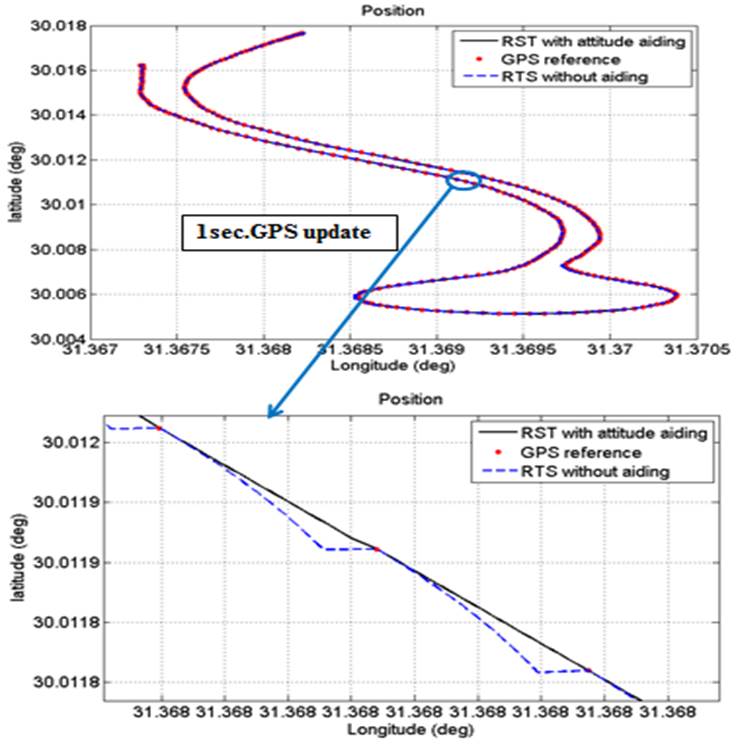
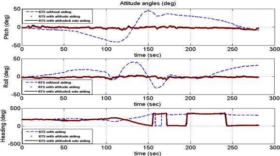
In the beginning, with respect to the real-time solution (RTS), we made a conventional INS/GPS integration-based UKF without any kind of aiding sensors and without any correction for the pitch and roll channels by the CF and we refer to this case by (RTS without aiding), then after that we applied the complementary filter regard the correction of pitch and roll channels; in addition, we used the magnetometer as an aid sensor for more accurate heading angle and we refer to this case by (RTS with attitude aiding). In case of RTS with attitude aiding, we found that the performance of the integrated system has been improved by make a comparison between the quantitative position errors for both cases such as standard deviation, mean, maximum error in east and north positions and the maximum horizontal error (MHE), these quantitative position errors were found decreased due to the enhancement which occurred in the attitude channels as shown in Table 1 and in Figure 9 which they represent the real time solution with and without attitude aiding. As an example, we noticed that the MHE is reduced by 45.354 % in case of RTS with attitude aiding. Furthermore, we noticed that the RTS of the attitude errors in pitch, Roll and Heading directions are depicted as shown in Figure 10. Figure 11 clarifies the enhancement of the navigation resultant trajectory in Latitude/Longitude because of the reduction in errors after using the improved attitudes in case of RTS with attitude aiding. All the results shown in figures prove that the proposed technique is promising and the estimated trajectory based on RTS with attitude aiding follow the reference trajectory without significant errors. It is an important to be mentioned here that the accuracy of UKF slightly more accurate than the EKF due to the low-dynamics of the land vehicle (EIdesoky et al., 2017b; LaViola, 2003). From Table 1 we can notice that the utilized extremely low-cost and grade of IMU as an inertial sensor is suitable for low-cost integrated navigation systems of land vehicle applications which tolerate a 2D position with a maximum horizontal error (MHE) of about 3.19 meters in case of GPS available.
Table 1 Position errors during navigation in case of 1sec. GPS update rate.
| Position errors (m) for 1sec. GPS update rate | |||||
| Mean | Std. | Max. Error | Max. Horizontal Error | ||
| RTS without aiding | East | 0.384 | 0.51 | 3.964 | 5.840 |
| North | 0.688 | 0.76 | 4.289 | ||
| RTS with attitude aiding | East | 0.227 | 0.24 | 1.899 | 3.1915 |
| North | 0.460 | 0.41 | 2.565 | ||
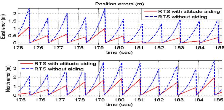
Figure 9 Position errors in east/north for GPS/INS integrated system in case of 1sec. GPS update rate.

Figure 10 Attitude errors in roll, pitch and azimuth for GPS/INS integrated system in case of 1sec. GPS update rate.
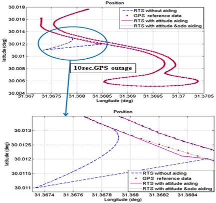
5.2. Navigation results during 10 sec GPS outage
In this section, we made a test to validate our proposed technique during the GPS denied environment by simulate a tunnel crossing or an urban canyon crossing via 10 second GPS data outage. In this case we noticed that the accumulated INS positioning errors increase rapidly during the outage interval. Then we started our proposed technique test based on a real time solution with attitudes and odometer aiding and we referred to this case by (RTS with attitude and odo aiding) , then we compared our proposed case with other two cases which are RTS without aiding and RTS with attitude aiding. In our proposed case in addition to using the attitude aiding we used the odometer sensor to collect the velocity measurements of the land vehicle instead of GPS velocity during the GPS outage. In case of RTS with attitude and odometer aiding we found that the performance of the integrated system has been improved as clearly shown in a comparison between the quantitative position errors such as standard deviation, mean, maximum error in east and north positions and the maximum horizontal error (MHE), these quantitative position errors were found decreased. As we notice from the comparison in Table 2 and as shown in Figure 12, we will find that The MHE is equal to 161.945 (m) during 10 second GPS outage without any kind of aiding then we will see that the position error dramatically damp due to the enhancement which occurred in the attitude channels after attitude aiding with the INS data and the MHE reduced by 87.205 %; while, after we added the measurement velocity from the odometer sensor and vehicle constrains to the aforementioned RTS with attitude adding then the MHE reduced by 92.74 % and this comparison clearly prove that the localization solution will be more accurate in case of our proposed technique when UKF integration done after using the improved pitch and roll angles as an output of CF and using the heading angle from the magnetic compass in addition to utilizing the velocity from the odometer velocity. Figures 13-14 show the improvements which happened in the navigation resultant and verify our proposed MSDF technique to be a suitable for solving the problem of real time land vehicle localization. From Table 2 we can notice that the utilized extremely low-cost and grade of IMU as an inertial sensor is suitable for low-cost integrated navigation systems of land vehicle applications which tolerate a 2D position with a maximum horizontal error (MHE) of about 11.75 meters in case of GPS not available.
Table 2 Position errors during navigation in case of 10sec GPS outage.
| Position errors (m) for 10sec. GPS outage | |||||
| Mean | Std. | Max. Error | Max. Horizontal Error | ||
| RTS without aiding | East | 1.789 | 9.81 | 116.2 | 161.945 |
| North | 1.96 | 9.17 | 112.8 | ||
| RTS with attitude aiding | East | 0.476 | 1.66 | 17.51 | 20.721 |
| North | 0.646 | 1.22 | 11.08 | ||
| RTS with attitude & odo. Aiding | East | 0.337 | 0.72 | 6.342 | 11.750 |
| North | 0.623 | 1.09 | 9.892 | ||

6. Conclusions
In this paper a real time nonlinear MSDF solution based on extremely low-cost and grade inertial sensor for land vehicle navigation system is presented. The utilized low-cost inertial sensor-based MEMS are IMU, commercial GPS, CAN bus (OBD) shield which senses the vehicle velocity and digital magnetic compass sensors. Loosely coupled integration architecture based on two platforms of 32-bit ARM core microcontroller and one platform of 16-bit AVR ATMEL microcontroller using UKF has been implemented. The integrated mechanism has been implemented and its performance has been evaluated through real time experimental work and post-processing domain.
A complementary filter (CF) has been implemented to improve the tilt angle drift. In case of available GPS conditions, the performance of the integrated system and the accuracy of the estimated localization state have been improved by using the RTS method with attitude aiding and the MHE errors reduced by 45.354 %. In case of GPS-denied environments, the proposed integrated mechanism based on RTS with attitude and odometer with vehicle constrains aiding is presented and the MHE reduced by 92.74 %. The proposed mechanism overcome the rapidly increasing navigation errors due to GPS outage and ensure a land vehicle continuous navigation solution with high performance accuracy comparable with RTS without aiding technique and RTS with attitude aiding technique. The results of the real-time experiment show the performance of the proposed technique based on UKF applied to the nonlinear system without linearization of the state model. Finally, the paper showed that the low-cost hardware based on ARM core microcontroller can handle the computational complexity of performing the unscented transformation process and the calculations of the proposed algorithm with good output navigation results compared with the reference trajectory.

