


 text new page (beta)
 English (pdf)
 Article in xml format
 Article references
 Send this article by e-mail
 Cited by SciELO
  Similars in
SciELO
Similars in
SciELO 
 Permalink
1. Introduction
This study examines a vendor-buyer coordinated system featuring batch fabrication, outsourcing, quality reassurance, discontinuous deliveries, and an unreliable machine. Most real-life manufacturing systems experience unanticipated nonconforming items and breakdowns. As such instances occur, corrective action and rework/disposal of nonconforming items must be undertaken to avoid delay in the fabrication schedule and attain the desired product quality. Vinod and Solberg (1984) examined the single- and multi-stage unreliable fabrication systems using queueing models. The authors derived the exact solution for the queueing model with a single-stage and presented two approximations for the closed network queueing model with multiple stages. Their approximation results/performances were validated/compared against the exact solution in the literature. Groenevelt, Pintelon, and Seidmann (1992) studied an unreliable fabrication facility with safety stocks and batch production, wherein a constant failure rate and random failure-repair time of the facility were assumed. Diverse bounds of service-level were examined to find their impacts on different system variables. A production control discipline was proposed to investigate the relationship between the safety stocks and the renewal process of a particular type of single server queue. The authors also showed how their approaches could be applied to broader decision makings in resource allocation fields. Dohi, Okamura, and Osaki (2001) considered an economic manufacturing quantity (EMQ) model with preventive maintenance, stochastic facility breakdowns, (PM), and safety stocks. Their purpose was to jointly decide the optimal control policies of the PM schedule and the quantities of safety stocks that keep the total cost at a minimum. Besides, the authors found out that both the safety stocks and total cost rise as breakdown rate increases. Chakraborty, Giri, and Chaudhuri (2009) studied the production lot-size problem considering breakdowns and different inspection schedules for a deteriorating process. Corrective action of breakdown situation and preventive maintenance are undertaken accordingly. The authors proposed models based on general shift and various distributions of machine failure and repair times to derive a suboptimal lot-size policy. Numerical examples were offered to show the results’ applicability and sensitivity analyses on system performances with/without inspection policy. Goerler and Voß (2016) used a mixed-integer programming approach to explore the capacitated batch-size problem with defective products and rework processes. Various numerical experiments were performed to explore the influences of changes in defective instances on the required computer times for obtaining the optimal batch-size solutions. Additional works (Al-Bahkali & Abbas, 2018; Arun, Lincon, & Prabhakaran, 2019; Ghalme, Mankar, & Bhalerao, 2017; Richter, 1996; Saari & Odelius, 2018; Sarker, Jamal, & Mondal, 2008; Shakoor, Abu Jadayil, Jaber, & Jaber, 2017; Souha, Soufien, & Mtibaa, 2018; Vujosevic, Makajic-Nikolic, & Pavlovic, 2017; Zahraee, Rohani, & Wong, 2018) studied the impact of various characteristics of unreliable facility and rework/disposal of defective products on fabrication systems and operations management.
Production managers apply an outsourcing strategy to effectively reduce fabrication uptime or release in-house facility’s workloads. Vining and Globerman (1999) presented a conceptual structure for comprehending the correct and less risky outsourcing decision. Specifically, through identifying the pre- and post-outsourcing risks and implementing certain suggested strategies to avoid or lessen those potential risks in advance (or pre-outsourcing stage). The authors referred to transaction costs in the literature to support their conceptual framework. De Fontenay and Gans (2008) considered a bargaining perception on strategic subcontracting and supply competition, wherein the subcontracting decision of a downstream company and its upstream fabrication resources is involved. The authors portrayed a downstream company has a choice to either subcontract to a reputable upstream company or a new and independent firm. Hence, it faces a trade-off between the higher resource value linked to those who could consolidate upstream capabilities and the lower input costs afforded by an independent competition. The result of their study indicates that outsourcing to an established firm is more beneficial. Rosar (2017) explored the connection between strategic subcontracting and optimal purchase policy. First, a subcontracting choice that relies on a non-cost-savings mechanism was presented and analyzed. Then, the author extended it to a cost-savings relating rationale, with the discussion of the incentives of sellers who employ in nested subcontracting policies. Additional works (Chiu, Liu, & Hwang, 2017; Chiu, Chiu, Lin, & Chang, 2019a; Mohammadi, 2017; Skowronski & Benton, 2018) investigated the impact of distinct outsourcing characteristics on the manufacturing systems and enterprise management.
In real supply-chain environments, the transportation of goods is commonly planned using multi-shipment at specific time intervals. Thomas and Griffin (1996) examined the conventional business processes in the stages of procurement, fabrication, and distribution, and indicated the need for coordinating these stages as a supply chain. The authors suggested taking advantage of recent progress in advance communication technology to place specific emphasis on the effective management of the coordinated supply-chain model to reduce overall operating costs. Swenseth and Godfrey (2002) examined the stock refilling decisions incorporating certain transportation cost functions from the literature and showed that no unnecessary complexity was added to the decision process, nor loss in accuracy of the decision. Farsijani, Nikabadi, and Ayough (2012) employed the simulated annealing methodology to explore a multiproduct economic production quantity (EPQ) model with discrete shipping orders and space constraints. Their batch- production model also considered realistic factors such as the imperfect manufacturing process, rework of defective stocks, and allowable shortages. The LINGO package helped solve the linear examples, and the simulated annealing methodology assisted in resolving the non-linear combinatorial optimization examples. Montarelo, Glardon, and Zufferey (2017) used the Tabu searching metaheuristic to investigate a four-echelon stock management decision in a decentralized supply chain setting. The authors proposed a global simulation methodology and set different service levels to deal with the market’s random demands, to explore/optimize the four-echelon linear/nonlinear supply chains. Their result showed that there are substantial differences among echelons in crucial stock and cost parameters. The authors claimed their approach could be generalized for boarder applications. Additional works (Arabi, Dehshiri, & Shokrgozar, 2018; Bolaños, Escobar, & Echeverri, 2018; Chiu, Wu, & Tseng, 2019b; Morales, Franco, & Mendez-Giraldo, 2018; Nielsen & Saha, 2018; Paz, Granada-Echeverri, & Escobar, 2018; Puška, Kozarević, Stević, & Stovrag, 2018; Stažnik, Babić, & Bajor, 2017; Zhao, Qian, Nakamura, & Nakagawa, 2018) studied the influence of distinct features of multiple deliveries on various types of manufacturing-transportation and supply-chain systems. Few prior works have investigated the joint influence of breakdowns, outsourcing, multiple deliveries, and rework/disposal of defective stocks on the optimal batch-fabrication runtime decision, this work aims to fill the gap.
2. The proposed model
This study determines the optimal hybrid inventory replenishment runtime for a vendor-buyer coordinated system with the breakdown, outsourcing, multiple deliveries, and rework/disposal of defective items. Suppose the annual demand rate λ of a manufactured product is supplied by a vendor at a fabrication rate of P1 units per year in a vendor-buyer coordinated system. To shorten fabrication uptime of the batch production plan, the vendor decides to outsource a π portion of the batch size Q (where 0 < π < 1). Thus, Kπ and Cπ denote the fixed and unit costs relating to the vendor’s outsourcing policy. The relationship between outsourcing relevant parameters and their corresponding in-house variables is shown as follows:
where C and K represent the in-house fabrication unit and setup cost, respectively; and β2 and β1 denote the relating ratios between these variables. It is noted that when π = 1, our model turns into a “buy” rather than “make” model; in contrast, when π = 0, the proposed model becomes a purely in-house production model.
The in-house fabrication process may produce an x portion of nonconforming items randomly, at a rate d 1 (where d 1 = xP 1 and P 1 stands for the in-house manufacturing rate). To prohibit the stock-out situation, we assume that (P 1 - d 1 - λ) > 0. Careful inspection of the nonconforming items separates the rework-able from the scrap (where the scrap ratio θ1 among the nonconforming is assumed). In each batch fabrication cycle, a rework process immediately follows the regular manufacturing process, at a reworking rate of P 2 and an extra cost C R is associated with each reworked item. Also, we assume an imperfect rework process, a scrap ratio θ2 among the reworked items exists. Hence, the overall scrap rate is φ (which sums up to (θ1 + (1 - θ1) θ2) in each cycle, and all scraps are disposed with unit disposal cost C S. As to the outsourced products, we assume that their quality is guaranteed by the outside provider, and they are scheduled to be received at the end of the in-house rework process, before the beginning of the delivery time of finished goods.
Moreover, the in-house production machine is not reliable, it is subject to random failure (which follows the Poisson distribution, with β as mean per year). When a failure occurs (as shown in subsection 2.1), a specific abort/resume stock controlling policy is used. Its guideline is to instantly repair the failure and promptly resume fabrication of the interrupted/unfinished lot when the machine is restored. A constant failure repair time t r is assumed; in case that actual repair time is greater than t r, a piece of rental equipment will be put in use to avoid further delay in production. Upon completion of the fabrication and rework processes, and receipt of outsourced items, n equal-size installments of the lot are shipped to the buyer at fixed time interval t' nπ during distribution time t' 3π. The additional notation used in this study is listed below.
t- |
time before a random failure occurs (in years), |
Q- |
batch size, |
M- |
machine repair cost, |
t1π- |
uptime in the proposed hybrid replenishment vendor-buyer coordinated system with random failure and quality assurance - the decision variable, |
t'2π- |
rework time in the failure occurrence case, |
T'π- |
cycle length in the failure occurrence case, |
d2- |
production rate of scrap items during t' 2π, |
h- |
perfect item’s unit holding cost, |
h1- |
reworked item’s unit holding cost, |
h2- |
buyer stock’s unit holding cost, |
h3- |
safety stock’s unit holding cost, |
C1- |
safety stock’s unit cost, |
CT- |
unit transportation cost, |
K1- |
fixed transportation cost, |
g- tr, |
fixed machine repair time, |
D- |
quantity per delivery, |
I - |
the leftover stocks in each delivery time interval, |
H0- |
level of perfect stocks when a failure occurs, |
H1- |
level of perfect stocks when the fabrication process ends, |
H2- |
level of perfect stocks when the rework process ends, |
H- |
level of perfect stocks after receipt of outsourced items, |
I(t)- |
level of perfect stocks at time t, |
IF(t)- |
level of safety stocks at time t, |
Id(t)- |
level of nonconforming stocks at time t, |
Is(t)- |
level of scrap at time t, |
Ic(t)- |
level of buyer’s stocks at time t, |
TC(t1π)1 = |
total system cost per cycle in the failure occurrence case, |
E[TC(t1π)1] = |
the expected total system cost per cycle in the failure occurrence case, |
E[T'π] = |
the expected cycle length in the failure occurrence case, |
t2π- |
rework time in the case of no failure occurrence, |
t3π- |
stock delivery time in the case of no failure occurrence, |
tnπ |
time interval between any two deliveries in the case of no failure occurrence, |
Tπ |
cycle length in the case of no failure occurrence, |
TC(t1π)2 = |
total system cost per cycle in the case of no failure occurrence, |
E[TC(t1π)2] = |
the expected total system cost per cycle in the case of no failure occurrence, |
E[TCU(t1π)] = |
the expected system cost per unit time for the proposed system with or without failure occurrence, |
E[T’π] = |
the expected cycle length in the case of no failure occurrence, |
t1- |
uptime for the proposed system without breakdown, nor outsourcing, |
t2- |
rework time for the proposed system without breakdown, nor outsourcing, |
t3- |
delivery time for the proposed system without breakdown, nor outsourcing, |
T- |
cycle length for the proposed system without breakdown, nor outsourcing, |
Tπ- |
replenishment cycle length for the proposed system with or without failure occurrence. |
The following subsections examine two distinct cases due to the random failure in the proposed model:
2.1. Case 1: A random failure occurs during fabrication uptime
2.1.1. During the fabrication process of Case 1
Figure 1 shows the level of perfect inventories in this case (i.e., t < t1π), wherein at the time when a failure happens, the level of inventory reaches H0 and once the failure is repaired, it continues to pile up to H1 at the end of uptime and reaches H2 at the end of rework process. Then, the outsourced items are received and the level of the perfect stock reaches to H, before the beginning of product distribution time t'3π.

Figure 1 Level of perfect inventories in the proposed hybrid inventory replenishment vendor- buyer coordinated system with random breakdown and quality reassurance (in brown) as compared to the proposed system without breakdown, nor outsourcing (in black).
Figure 2 displays the on-hand level of safety stock in the proposed system. It indicates that in the failure occurrence case, the safety stock will be added to the finished batch and delivered in t'3π for meeting extra buyer’s demand during tr.

Figures 3 and 4 illustrate the levels of nonconforming and scrap items in the proposed system with failure occurrence, respectively.
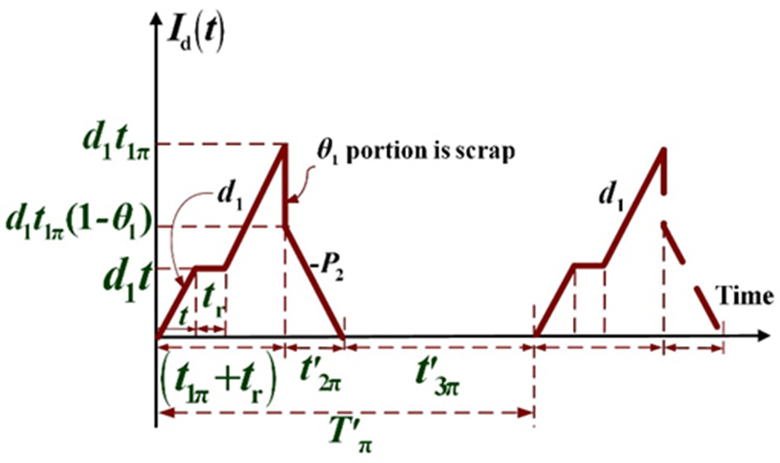

Based on the aforementioned description of the in-house fabrication process, one can observe the following straightforward equations (please refer to Figures 1 to 5):

Figure 5 Level of perfect inventories in the proposed hybrid inventory replenishment vendor- buyer coordinated system with quality reassurance, but no machine breakdown (in brown) as compared to the same system without outsourcing option (in black).
2.1.2. During the delivery time of Case 1
Total delivery quantity H at the beginning of product distribution time t'3π must include λtr as shown in Eq. (12). Total inventories during the product distribution time t' 3π (Chiu et al., 2019b) is exhibited in Eq. (13).
2.1.3. The status of buyer’s stocks in Case 1
Total inventories at the buyer side during the cycle length T' π can be calculated (Chiu et al., 2019b) as shown in Eq. (14).
2.1.4. Total cost per cycle for Case 1
Total cost per cycle in failure occurrence case, TC(t 1π)1 comprises both the variable and fixed outsourcing and in-house fabrication costs, machine repaired cost, safety stock relevant costs (see Fig. 2), both fixed and variable shipping costs, rework and disposal costs, and total holding costs (including perfect items, nonconforming and reworked items, and buyer’s stocks) during the entire cycle, as shown in Eq. (15).
Substitute Equations (1) to (14) in Eq. (15), and use the expected value to cope with the randomness of x, the expected total system cost per cycle in the failure occurrence case E[TC(t 1π)1] can be derived as follows:
where
2.2. Case 2: No machine failure occurrence during fabrication uptime
Figure 5 displays the level of perfect inventories in this case (i.e., t ≥ t 1π). Since no failure occurs, the inventory level goes up to H 1 when uptime ends and it reaches H 2 when rework is completed. Upon receipt of the outsourced items, the level of perfect inventories reaches H, before the beginning of product distribution time t 3π.
Since no machine failure occurs, the safety stock remains unused throughout the cycle length T π. The following straightforward equations for this no failure occurrence case can be directly observed:
Equations (10) and (11) remain valid in this case, and the inventories in distribution time t 3π and at the buyer side in T π can be computed using formulas shown in Eqs. (24) and (25) (Chiu et al., 2019b).
2.2.1. Total cost per cycle for Case 2
Total cost per cycle in no failure occurrence case, TC(t 1π)2 comprises both the variable and fixed outsourcing and in-house fabrication costs, safety stock holding cost (see Fig. 8), rework and disposal costs, transportation costs (both variable and fixed costs), and total holding costs (including reworked, perfect items, and nonconforming items, and buyer’s stocks) during the entire cycle, as shown in Eq. (26).
Substitute equations (17) to (25) and (10) to (11) in Eq. (26), and use the expected value to cope with the randomness of x, the expected total system cost per cycle for case 2, E[TC(t 1π)2] can be derived as follows:
3. Solution processes to the problem
Because of the assumption of Poisson distributed failure rate β per year, the time to failure obeys an Exponential distribution with f(t) = βe-βt (i.e., the density function) and F(t) = (1 - e-βt) (i.e., the cumulative density function). Also, since the scrap rate φ is random, hence, the cycle length is not constant.The renewal reward theorem is employed to cope with the variable cycle length. Therefore, E[TCU(t1π)] can be computed as follows:
where E[ T π], E[T' π], and E[T π] represent the following:
Substitute formulas (16), (27), and (29) in formula (28), along with extra efforts in derivations, one can obtain E[TCU(t 1π)] as follows (for details please refer to Appendix A):
The first and second derivatives of E[TCU(t 1π)] are shown in equations (B-1) and (B-2) in Appendix B. Since the first term on the right-hand side (RHS) of Eq. (B-2) is positive, it follows that the E[TCU(t 1π)] is convex if the second term on the RHS of Eq. (B-2) is also positive. That means if γ (t 1π) > t 1π > 0 holds (see Eq. (B-3) for details).
Once Eq. (B-3) is verified to be true, we can solve the optimal t 1π * by setting the first derivative of E[TCU(t 1π)] = 0 (refer to Eq. (B-1)). Since the first term on the RHS of Eq. (B-1) is positive, we obtain the following:
Let z 0, z 1, and z 2 represent the following:
Then, we can rearrange Eq. (33) as follows:
Apply the square roots solution, t π * can be found as follows:
As the cumulative density function of Exponential distribution F(t 1π) = (1 - e -βt1π ) is throughout for [0.1], so does its complement e -βt1π . Moreover, Eq. (33) can be rearranged as follows:
To solve the optimal t 1π *, we start with letting e-βt1π = 0 and e-βt1π = 1, then compute Eq. (35) to find the bounds for t 1π (i.e., t 1πU and t 1πL). Next step use present t 1πU and t 1πL to compute and obtain update values of e-βt1π and e-βt1π. Re-compute Eq. (35) using the current e-βt1π and e-βt1π to obtain the update bounds t 1πU and t 1πL. If (t 1πU = t 1πL) holds, then, t 1π * is derived (i.e., t 1π * = t 1πU = t 1πL); otherwise, repeat the above-mentioned steps, until it holds.
4. Numerical example
The following numerical example demonstrates the applicability of our obtained result. The assumed values of system variables in this example are shown in Table 1.
Table 1 Assumed of values of system variables
| β | K1 | Cπ | λ | C | C1 | β2 | P1 | Kπ | CR | K | CS | CT | h2 |
| 1 | 90 | 2.8 | 4000 | 2.0 | 2.0 | 0.4 | 10000 | 60 | 1.0 | 200 | 0.3 | 0.01 | 1.6 |
| π | n | θ1 | M | θ2 | h3 | β1 | P2 | x | φ | g | h | h1 |
First, we verify if E[TCU(t 1π)] is convex (i.e., whether Eq. (B-3) holds). Since e -βt1π falls within the interval of [0, 1], let e -βt1π = 0 and e -βt1π = 1, and apply Eq. (35) to gain t 1πU = 0.2875 and t 1πL = 0.0909 initially. Then, use t 1πU and t 1πL to calculate e -βt1πU and e -βt1πL . Finally, apply Eq. (B-3) with the present values of e -βt1πL , e -βt1πU , t 1πL, and t 1πU to confirm that γ(t1πL) = 0.3103 > t1πL = 0.0909 > 0 and γ(t1πU) = 0.5320 > t1πU = 0.2875 > 0, respectively. Therefore, the convexity of E[TCU(t1π)] is assured for β = 1.0, and optimal t1π* exists. Additionally, a wider range of β values have been used to test for convexity of E[TCU(t1π)] to demonstrate the boarder applicability of the obtained result from this study (see Table 2)
Table 2 Verification of convexity of E[TCU(t1π)] against different βs.
| β | γ(t1πU) | t1πU | γ(t1πL) | t1πL |
| 10 | 0.7927 | 0.2844 | 0.0467 | 0.0216 |
| 8 | 0.6141 | 0.2845 | 0.0573 | 0.0263 |
| 6 | 0.4998 | 0.2847 | 0.0744 | 0.0336 |
| 5 | 0.4621 | 0.2848 | 0.0874 | 0.0389 |
| 4 | 0.4370 | 0.2850 | 0.1060 | 0.0461 |
| 3 | 0.4268 | 0.2853 | 0.1346 | 0.0561 |
| 2 | 0.4415 | 0.2858 | 0.1851 | 0.0703 |
| 1 | 0.5320 | 0.2875 | 0.3103 | 0.0909 |
| 0.5 | 0.7277 | 0.2909 | 0.5215 | 0.1044 |
| 0.01 | 6.0228 | 0.5277 | 5.6043 | 0.1200 |
To solve the optimal t 1π *, we start with letting e -βt1π = 0 and e -βt1π = 1 and apply Eq. (35) to gain the bounds for t 1π (i.e., t 1πU = 0.2875 and t 1πL = 0.0909). Next, we repeatedly use resent t 1πU and t 1πL to compute and update values of e -βt1πU and e -βt1πL , and re-compute Eq. (35) using current e -βt1πU and e -βt1πL until t 1πU = t 1πL = t 1π *. Table 3 exhibits the step-by-step results for searching t 1π *. Therefore, the optimal uptime for this example t 1π * = 0.1224 and E[TCU(t 1π *)] = $12,542.25.
Table 3 Step-by-step results for searching t1π*.
| Step # | t1πU | e-βt1πU | t1πL | e-βt1πL | t1πU - t1πL | E[TCU(t1πU)] | E[TCU(t1πL)] |
| - | - | 0 | - | 1 | - | - | - |
| 1 | 0.2875 | 0.7501 | 0.0909 | 0.9131 | 0.1966 | $13,371.17 | $12,637.28 |
| 2 | 0.1539 | 0.8573 | 0.1151 | 0.8913 | 0.0388 | $12,598.72 | $12,546.23 |
| 3 | 0.1292 | 0.8788 | 0.1207 | 0.8863 | 0.0085 | $12,545.38 | $12,542.44 |
| 4 | 0.1239 | 0.8835 | 0.1220 | 0.8851 | 0.0019 | $12,542.41 | $12,542.26 |
| 5 | 0.1227 | 0.8845 | 0.1223 | 0.8849 | 0.0004 | $12,542.26 | $12,542.25 |
| 6 | 0.1224 | 0.8848 | 0.1224 | 0.8848 | 0.0000 | $12,542.25 | $12,542.25 |
4.1. Impact of core system feature on the problem
The convexity of E[TCU(t 1π)] and the initial bounds for t 1π is exhibited in Figure 6.

Figure 7 illustrates the impact of variations in φ along with various x values on E[TCU(t1π*)]. It indicates that as both φ and x rise, E[TCU(t1π*)] increases noticeably.

The influence of changes in mean-time-to-breakdown 1/β on E[TCU(t1π*)] is displayed in Figure 8. It shows our optimal solution E[TCU(t1π*)] = $12,542 (for x = 0.2 and n = 3), it also specifies that as 1/β increases to over 0.17, E[TCU(t1π*)] begins to decline significantly; and as 1/β rises to extremely large (e.g., 1/β ≥ 100), E[TCU(t1π*)] = $11,962 (i.e., the same result as what is obtained from a problem without breakdown occurrence).

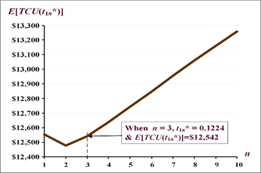
The impact of differences in the number of deliveries n (per cycle) on E[TCU(t 1π*)] is depicted in Figure 9. It shows our optimal solution given n = 3, it also indicates that when n = 2 we have the minimal E[TCU(t 1π*)], and as n increases, E[TCU(t 1π*)] goes up significantly.
The effect of variations in the outsourcing portion π on utilization is demonstrated in Figure 10. It shows that utilization noticeably decreases as π increases; and for π = 0.4 (as we assumed in our example), utilization declines from 47.72% to 28.11%.

The breakup of E[TCU(t 1π *)] of our example is exhibited in Figure 11. It reveals the sum of outsourcing relevant setup and variable costs is 37.7%; total in-house relevant costs are 51.1% (including quality and breakdown related expenses), and supply chain relevant cost (including delivery and buyer’s holding costs) adds up to 11.2%.

The influence of changes in the number of deliveries n (per cycle) on the delivery and stock holding costs is illustrated in Figure 12. It reveals that as n increases, the fixed product distribution cost goes up significantly and in-house holding cost rises accordingly (the latter is simply due to a slow stock movement from the vendor to the buyer when n increases); on the contrary, the buyer holding cost drops accordingly.

4.2. The joint impact of the core system features on the problem
The joint impact of differences in uniformly distributed nonconforming rate x and total scrap rate φ on the optimal decision variable t1π* is explored and illustrated in Fig. 13. It shows that t1π* increases significantly as both x and φ rise.

The combined influence of variations in the outsourcing portion of a batch π and mean time to breakdown 1/β on the optimal decision variable t1π* is studied and depicted in Fig. 14. It reveals that t1π* decreases enormously as π increases, especially when 1/β value is less than 0.17; and as 1/β increases to over 0.17 and π < 0.45, t1π* declines noticeably.

The joint effect of changes in the meantime to breakdown 1/β and total scrap rate φ on E[TCU(t1π*)] is demonstrated in Fig. 15. It shows E[TCU(t1π*)] decreases considerably as 1/β increases and as φ goes up, E[TCU(t1π*)] increases slightly. The effect of 1/β on E[TCU(t1π*)] is more significant than that from φ.

4.3. Discussion and limitation
This study develops the inventory replenishment model based on a case where only one or no breakdowns occur during a production cycle. Table C-1 (see Appendix C) presents the Poisson probabilities results for a machine with different mean breakdown rates per year. It specifies that for a machine in good condition, or with an average of less than one breakdown occurrence per year, this study is appropriate, as there is over 99.31% chance that only one or no breakdowns will occur (refer to Table C-1).
Besides, for a machine in fair condition, or with an average of less than or equal to two breakdown occurrences per year, our model indicates that there is over 97.27% chance of one or no breakdowns occurring (see Table C-1). However, to explore the fabrication planning for a piece of equipment having a mean breakdown rate greater than five per year, the suitability of our model will fall below 80%, therefore, a different model must be developed for this specific condition.
5. Conclusions
This study aims to assist multinational/translational manufacturing firms with making the accurate decisions in their intra-supply chain environments, enable competitive strategies (including quality, low-cost, and timely delivery), and cope with the realities of limited capacity and unreliable equipment. Therefore, we examine a vendor-buyer coordinated system featuring batch fabrication, outsourcing, multiple deliveries, rework/disposal of defective items, and Poisson distributed breakdowns. Using the modeling, formulation, derivation, and optimization procedure along with a recursive algorithm, we in sequence obtain the problem’s cost function, justify its convexity, and find the problem’s optimal replenishment runtime. A numerical illustration is offered to show the applicability of the result that reveals various key system characteristics/capabilities, such as the distinct and joint influences of breakdowns (see Figs. 8, 11, 14, and 15), outsourcing (Figs. 10, 11, and 14), rework/scrap (Figs. 7, 11, 13, and 15), and delivery-frequency factors (Figs. 9, 11, and 12) on various system parameters, performance, and optimal runtime (Fig. 6). The methods proposed here and their results can facilitate managerial operations planning and strategic decision-making in an intra-supply chain setting in practice.

