


 text new page (beta)
 English (pdf)
 Article in xml format
 Article references
 Send this article by e-mail
 Cited by SciELO
  Similars in
SciELO
Similars in
SciELO 
 Permalink
1. INTRODUCTION AND BACKGROUND
Various aspects may influence the occurrence of traffic accidents as they have many complex causes, globally divided into three main elements: the road user, the road features and the vehicle, where the road user is the main contributing factor, responsible for up to 95% of accidents (Downing, Baguley, & Hills, 1991; Norman, 1962).
Traffic Accidents (TAs) are estimated as the ninth leading cause of fatality in the world with a similar risk to that caused by many diseases. More than 1.2 million people die every year on roads around the world and thousands more suffer injuries resulting from traffic crashes. Young people at a working age, between 15 and 29 years oíd, are the most common victims (World Health Organization, 2015).
In Brazil, TAs are responsible for more than 40,000 fatalities annually. From 1996 to 2012, the Ministry of Health (MH) registered more than half a million fatalities due to traffic accidents (DATASUS, 2014). Sáo Paulo is the Brazilian state with the largest economy and the most populous, where 21.56% of the country's inhabitants are concentrated (IBGE, 2010). Moreover, it is state with the highest absolute number of traffic fatalities: in 2012, there were 7,003 fatalities, a rate of 16.71 fatalities per hundred thousand inhabitants (DATASUS, 2014).
Understanding the causes of traffic accidents involves several factors related to the three main elements mentioned previously, as well as the environment in which they happen. These factors can be better understood and investigated by applying classification algorithms. A Decisión Tree (DT) is an example of an analysis that explores a large data set in order to find patterns among the variables using nonparametric classification algorithms.
In some studies, DT algorithms have been used to characterize patterns through classification rules for accident occurrence frequency and even to classify the injury severity (Abellán, López, & De Oña, 2013; Chang & Chen, 2005; Chang & Wang, 2006; De Oña, López, & Abellán, 2013; López, De Oña, & Abellán, 2012).
A study conducted by Chang and Cheng (2005) collected data on accidents that occurred during 2001 and 2002 on one of the most important roads in Taiwan. Classification And Regression Tree (CART) algorithm and negative binomial regression models were developed to establish a link between the accidents and the variables: road geometry, traffic characteristics and environmental factors. When comparing the prediction performance between the DT and the negative binomial regression models, the study showed that the CART algorithm is a good alternative method to analyze the road accident frequency. CART results indicated that the average daily traffic volume and rain were key variables in road accident frequency.
A DT model, using the CART algorithm, was developed to establish the relationship between the injury severity in traffic accidents and the characteristics of the driver, the vehicle, the road, the variables related to the environment and the accident type, based on accident data from 2001 in Taipei, Taiwan. As noted by Chang and Wang (2006), pedestrians, motorcyclists and cyclists are the most vulnerable groups on a road.
A study carried out by López et al. (2012) used data from traffic accidents on rural roads in Granada (Spain) from 2004 to 2008. The analysis consisted of accident data with only one vehicle involved (a total of 1,801 records).The CART algorithm was the method used to build a model which included variables that contributed to the accident injury severity: the accident characteristics, the environmental information, the driver's characteristics and the road. The model found that male drivers are the main victims of accidents involving fatality or serious injuries. On the other hand, these types of accidents are more likely to occur with women when road lighting conditions are non-existent or insufficient.
To identify the main factors that contribute to the occurrence of crash severity, De Oña et al. (2013) showed an application with DT modeling. Accident analysis on rural roads in Granada (Spain) from 2003 to 2009 showed that the methods used in the DT approach, with CART and C4.5 algorithms, made it possible to classify the accidents based on the severity. These two algorithms also indicated that women have a higher risk of severe accidents when there is non-existent or insufficient lighting conditions. DT models are an alternative to parametric models as they identify data patterns and can be used to determine the interactions between the variables without strict mathematical assumptions or constraints such as population distribution, error independence, multicollinearity or constant variance.
Montella, Aria, D'Ambrosio, and Mauriello (2012) used DT and association rules to find relations between crash characteristics of powered two-wheelers and diverse variables. The objective was to detect unexpected relations to improve safety strategies. Kashani, Rabieyan, and Besharati (2014) developed a study to identify factors that influence the severity of passenger accidents and used the CART method to investígate the deaths of motorcycle passengers. The algorithm identified the área type, land use and the body part injured as the most important variables.
Another interest in studies related to road safety has been the use of macro-level data sets. In general, these studies use socio-economic and demographic characteristics, geographical data and/or other macro level information to analyze the impact on the results of models, as well as contributions to transport planning (Huang, Song, Xu, Zeng, Lee, & Abdel-Aty, 2016; Jiang. Abdel-Aty, Hu, & Lee, 2016; Khondakar et al., 2010; Lee, Abdel-Aty, & Cai, 2017; Lovegrove & Sayed, 2006; Wang et al., 2017). Studies such as Tolón-Becerra, Lastra-Bravo, Flores-Parra (2013), Lee et al. (2017) and Bougueroua & Carnis (2016) analyzed traffic accidents or fatality occurrence also including macro level variables in their models.
Huang et al. (2016) compared macro and micro models to predict zonal crash. They used a three year dataset from a Florida (US) urban road network and applied the macro-level Bayesian spatial model with conditional autoregressive prior and the micro-level Bayesian spatial joint model. The authors concluded that micro-zone models are better to predict specific zonal crashes and present a better overall fit. On the other hand, macro zone models are better to identify area-wide problematic zones. These models also are enabled to use dataset with fewer details and to include information not related to traffic engineering such as population, road network and land use, which are not so easy to intégrate into a micro-zone model. The authors proposed to use these integrated models to take advantage of both.
Wang, Huang, and Zeng (2017) examined the effects of including macro level variables as demographic and trip characteristics in negative binomial models (NB) and random parameter negative binomial models (RPNB). The macroscopic variables helped to improve the fit of the tested models. One of the authors' conclusions indicated that some macro level variables should be considered to estímate risk collision and local crashes, as well as traffic volumes and road features.
Khondakar et al. (2010) tested the macrolevel Collision Prediction Model (CPM) transferability using the recommended guidelines from two entirely different spatial-temporal región data sets. An analysis of the results revealed that macrolevel CPM transferability was possible and no more complicated than microlevel CPM transferability.
Lee et al. (2017) used macro and micro-level data from geographic units in models to predict intersection crashes. The results of the different models showed the following variables as being significant: income, population density, proportion of young (15-25 years), elderly (75 years or older) age group, proportion of public transit, motorcycles or walking commuters.
Tolón-Becerra et al. (2013) analyzed road accidents in Spain and observed that the increase in income (GDP) and vehicle-kilometers produced a greater number of fatal accidents and fatalities. Bougueroua & Carnis (2016) found a positive relationship between the improvement of GDP and the number of road traffic accidents, Le., higher economic development worsens road safety.
Taking into account that DT algorithms have been used in road safety studies to classify factors associated with traffic accidents using disaggregated data and that it is difficult to obtain road accident individual data (micro level) in Brazil, this research proposes an exploratory approach using macro zone dataset (municipality). Therefore, the aim of this study is characterize the municipalities with high fatality rates due to traffic accidents, considering macro level data from cities in Sao Paulo state (Brazil).
This paper consists of four sections, besides this introduction. Section 2 describes the statistical techniques used and in Section 3, the method procedure and materials are presented. Section 4 describes the results and discussions. Finally, in Section 5, the main conclusions are drawn.
2. DESCRIPTION OF TOOLS
2.1 DECISION TREE (DT)
A Decisión Tree (DT) is a nonparametric supervised machine learning method used for classification (Categorical dependent variable) and estimation (Numerical dependent variable). The aim of a Classification Tree is to classify a datábase in a finite number of classes through hierarchical rules (Quinlan. 1983).
DTs are usually graphically represented as hierarchical structures, making them easier to interpret than other techniques (Rokach & Maimón, 2008). Each tree segment is called a node, as follows: (a) the segment that contains the data of all elements of analysis is the root node; (b) the following nodes, the root node subdivisions, are called child nodes; and (c) if the nodes are not divided, they are called leaf or terminal nodes.
The criteria for data división are dependent on the algorithms. The algorithm used to split the data into the tree models aims to identify the independent variables that provide máximum data segregation (node homogeneity) according to the dependent variable valué. Some of the algorithms of Decisión Tree modeling are C4.5 (Quinlan, 1983), CHAID - Chi-square Automatic Interaction Detector (Kass, 1980), CART - Classification And Regression Tree (Breiman et al., 1984) and QUEST - Efficient Statistical Tree.
The algorithm used in this article was the CART (Classification And Regression Tree). The trees constructed by the CART algorithm are suitable for nonlinear problems and achieve satisfactory results for numerical and categorical dependent variables (Breiman et al., 1984). The growth of the tree is binary so that the classes formed in a división are more homogeneous than the previous división. In a tree, there are many simpler subtrees, therefore the resulting tree may be pruned once the process is complete.
One of the CART data partition criteria is the Gini index, which measures the degree of the data heterogeneity. Therefore, it can be used to measure the impurity of a node (Breiman et al., 1984). If this index is equal to zero, the node is puré. On the other hand, when it approaches the valué of one, the node is impure, increasing the number of classes evenly distributed in this node. It is expected that the Gini index decreases for each DT deep layer and the nodes become more and more homogeneous. Thus, the larger the number of divisions and subdivisions, the smaller the Gini index valúes.
The Gini index uses the impurity function i(t), presented in Equation 1.
Assume that the dependent variable is categorical, represented by k an l, respectively. Hence, p (k|t) and p(l|t) and are conditional probabilities of class k and l given node t.
The difference between the Gini criterion for the parent node is the sum of the values for child nodes (weighted by the proportion of cases in each child) and appears on the tree as improvement. The chosen variable is one that ensures a partition corresponding to the highest amount of improvement.
2.1.1. Classification Rules
From the DT structure, decision or classification rules can be extracted that present useful information base don the data. The rules are presented by a conditional logic form such as: if "A" then "B", where "A" is a prior independent or a prior independent variable (or a set of them), and as a consequence "B" is a class of the categorical dependent variable.
Thus, the conditional logic form starts with "IF" in the root node and ends in child nodes with "THEN", which are associated with the resulting class (the most likely category of dependent variable).
All the branches have a rule. However two parameters are used to extract important rules, defined as population (Po) and class probability (P), where the percentage of the population of cases is in the node in relation to the total number of cases analyzed, and the class probability is the percentage of cases for each class of the dependent variable. The selected rules will be representative with the mínimum valúes of Po^ 1% and P^ 60% (López et al., 2012).
Observing an example of DT application, for the choice of glasses (A, B and C), three Classification Rules can be found verifying the terminal nodes 1, 2 and 3, respectively.
2.1.2 Variable Importance
The Measure of Importance M(X) of an independent variable X in relation to the final tree T is defined as the (weighted) sum across all splits in the tree of the ímprovements that X has when it is used as a splitter. The Variable Importance VI(X) of X is expressed in terms of a normalized quantity relative to the variable having the largest measure of importance. It ranges from 0 to 100, with the variable having the largest measure of importance scored as 100 (Breiman et. al., 1984).
2.1.3 Stopping Rules
A DT growing process is controlled by stopping rules. The node will not be split if (Breiman et al., 1984):
all cases in a node have identical valúes of the categories of the dependent variable (highest homogeneity);
all cases in a node have identical valúes for each independent variable;
the size of a node is less than the user-specified mínimum node size valué (number of observations);
the split of a node results in a child node whose node size is less than the user-specified mínimum child node size valué;
for the best split s* of node t, the irnprovernent
Furthermore, if the current tree depth reaches the user-specified máximum tree depth limit valué, the tree growing process will stop.
2.2 CLUSTER ANALYSIS
Due to the large variability observed from the variables corresponding to the original datábase, the authors proposed an aggregation of the numerical valúes of the variables in order to discretize them, classifying them, for example, as high, average or low valúes of a particular variable.
Thus, the Cluster Analysis technique was used for each of the original variables in order to transform them into discrete variables. The Cluster Analysis (CA), also known as conglomérate analysis is a set of algorithms and optimization methods whose purpose is to group objects according to their characteristics, forming homogeneous groups or clusters, according to certain criteria. The objects in each group tend to be similar between themselves and different from other objects in other clusters. Obtained clusters must present both an internal homogeneity (within each group) and a large external heterogeneity (between clusters). Therefore, if the clustering is successful, when represented in a graph, the objects in the clusters will be very cióse, and the different clusters will be far (Hair, Black, Babin & Anderson 2010).
CA is a technique to analyze interdependencies between variables, because it is not possible to determine in advance the dependent and independent variables. On the other hand, it examines interdependencies between the entire set of variables. To apply CA, the following is required:
Define the clustering problem;
Select the variables to be treated statistically;
Select a similarity measurement of the conglomerates: objects with more similarity to each other are clustered in the same conglomérate. However, the most distant or different objects belong to different clusters. There are several ways to measure the similarity between objects, but the most used is the Euclidean distance.
Define the clustering process which depends on the variables under study and the problem being discussed: clustering processes can be hierarchical and non-hierarchical. Hierarchical clustering is characterized by establishing a hierarchy or structure as a tree and can be agglomerative or divisive. While the non-hierarchical clustering, also called K-means clustering, initially determines or assumes a conglomeration center and then groups all the objects that are closer to the center than a pre-set valué;
Previously define or not the number of clusters;
Interpret the resulting clusters in terms of variables used to establish them and other important additional variables.
2.2.1 Two-step Cluster Algorithms
The TwoStep cluster method is a scalable cluster analysis algorithm designed to handle very large data sets. It can handle both continuous and categorical variables. It has two steps 1) pre-cluster of the cases (or records) into many small sub-clusters; 2) cluster the sub-clusters resulting from pre-cluster step into the desired number of clusters. It can also automatically select the number of clusters (Zhang, Ramakrishnan, & Livny, 1996). In this study, we used this procedure.
Considering this, the clusters are recursively merged until a single cluster is obtained with all registers. The process starts by defining a starting cluster for each of the sub-clusters produced in the pre-cluster step. All clusters are then compared and the pair of clusters with the smallest distance between them is selected and merged into a single cluster. This process repeats until all clusters have been merged. To obtain a five-cluster solution, simply stop merging when there are five clusters, and so on for the other numbers of clusters.
2.2.2 Cluster Numbers
In this study, the cluster number was obtained automatically. To determine the number of clusters automatically, the Two-step method uses a two-stage procedure that works well with the hierarchical clustering method. Firstly, BIC is calculated to each number of clusters within a specified range and is used to find the initial estímate for the number of clusters (Zhang et al.. 1996). Thus, the BIC is computed as Equation 2:
Where
and other terms defined as in Distance Measure. The ratio of change in BIC at each successive merging relative to the first merging determines the initial estímate. Let dBIC(J) be the difference in BIC between the model with J clusters and that with (.1 + 1) clusters
Then, the change ratio for model J is
If dBIC(1) < 0, then the number of clusters is set to 1 (and the second stage is omitted). Otherwise, the initial estímate for the number of clusters k is the smallest number for which R1 < 0.04. Besides, In the second stage, the initial estímate is refined by finding the largest relative increase in distance between the two closest clusters in each hierarchical clustering stage.
2.2.3 Distance Measure
There are two forms to measure the similarity using the Two-Step Cluster Method: Euclidean and Log-Likelihood distance. The Euclidean distance is used just for continuous variables and is measured by the Euclidean distance between the two cluster centers (Zhang et al., 1996).
The Log-Likelihood distance is used for continuous or categorical variables and is equivalent to a probability based distance. In the log-likelihood calculation, a multinomial distribution is assumed for categorical variables, or a normal distribution for continuous variables and it is also assumed that the variables and cases are independent from each other. Thus, the distance between two clusters is related to the decrease in the log-likelihood as they are combined into one cluster (Zhang et al., 1996).
3. MATERIALS AND METHOD
The dataset of this study originates from different Brazilian public databases with aggregated data of states and cities. After data processing, the variables were discretized with cluster analysis, and finally, the CART algorithm was applied. The data processing and methodological steps (Figure 1) are described as follows.

3.1 STUDY AREA
The study área consists of 645 municipalities in the state of Sao Paulo, Brazil, which are spread across 248 square kilometers, with approximately 35 thousand kilometers of road network (DER, 2014; IBGE, 2010) . The state is the most populous of the country and includes 22% of the entire population, corresponding to 44 million inhabitants (IBGE, 2010) .
Regarding the economy, Sao Paulo is the Brazilian state with the largest industrial participation. In 2013, the Gross Domestic Product (GDP) was equivalent to just over US$ 10,000 per capita (in current USD) (SEADE, 2015) .
In 2016, the state had more than 190,000 kilometers of highways but just about 16% were paved and 2.9% were two lañe (DER, 2015) . Concerning the highway network characteristics, in 2015 a study evaluated th(e conditions of 9,650 kilometers of Sao Paulo state highways and considered the general status of 54.1% of roads as "Great". Specifically about pavement and signaling, more than 60% of the extensión was also classified as "Great". However, considering the road geometry 23.4% and 22.3% of the road was classified as "Great" and "Good", respectively and almost 40% was classified as "Regular" (CNT, 2015) .
3.2 DATABASE AND DATA PROCESSING
The datábase for this study comprised data mostly obtained from public databases and the variables "number of trips" and "extensión of the road network" were obtained secondarily from original information. Considering that is an aggregated analysis by área, we used rates or Índices for the sake of comparison. Thus, the dependent variable, "number of road traffic fatalities" was used as number of fatalities per 100,000 inhabitants. The independent variables of fleet were divided per 1,000 inhabitants.
3.2.1 Dependent variable
Brazil does not have a datábase that considere road traffic accident information for the whole country or for each state. The main macro level data available relates to traffic deaths by the Ministry of Health. This is not a specific datábase about traffic accidents, and therefore it does not provide information about accident causes, road characteristics or weather conditions. This datábase consists of regular data from mortalities in the country, therefore the main information available is socio demographic data, as well as death cause and location.
The State and Local Health Departments collect the Death Certificates filled out by medical professionals and provide the Mortality Information System (MIS) with the information contained therein. These data are available online at the DATASUS website. One piece of information, the basic cause of mortality, is encoded with the International Classification of Diseases (ICD-10) according to rules established by the World Health Organization. Deaths caused by transport accidents correspond to the V00-V99 ICD-10 code. (DATASUS, 2014) . This study used data whose cause of mortality was traffic accident per municipality in Sao Paulo state, Brazil.
The data obtained in absolute numbers were transformed to a rate (number of mortality by 100 000 population), as mentioned previously, to each year. In the next step, the averages of 2008, 2009 and 2010 were calculated and these data were discretized using a clustering method, as presented in Section 3.3.
3.2.2 Independent variables
The independent variables used in the study are municipality aggregated variables relating to socio-economic development, population and road information (vehicle fleet, road networks and number of trips).
The Human Development Index (HDI) evaluates the Ufe quality and economic development of the population. The Municipal Human Development Index (MHDI) fits the global methodology of the HDI to the Brazilian context and to the availability of national indicators to assess the development of the municipalities (Atlas Brasil. 2015) . Its rating was established by the United Nations ranging from 0 to 1, where 0 is very low and 1 is very high (Figure 2) and it was maintained in this study.

Fig. 2 Classification of Municipal Human Development Index limits. Source: Adapted from Atlas Brasil (2015).
The original demographic and socioeconomic data are from the 2010 Census (IBGE, 2010), as follows: área (in square kilometers), population, income, number of employed people and Gross Domestic Product (GDP). From these data, only área and GDP were selected in the DT as primary splitters. Population can be found in the dependent variable and vehicle fleet variable, both as rates. The other datasets, income and employed people, are included in the number of trips.
The number of trips was calculated based on the gravity model previously calibrated by Isler (2015) to estimate the number of annual trips by car between municipalities in the Southeastern Brazilian región, according to Equation 6.
Where: POP: population; RENDA: Income; OCUP: employed people and (d): road distance between cities in kilometers.
Vehicle fleet data were obtained from the National Traffic Department - DENATRAN that periodically makes this information available. In this study, we considered the following vehicle fleets: cars, trucks, motorcycles and similar vehicles, buses and minibuses. All data are by municipality and from 2010. The extensión of the highway network was obtained by geo-referenced data provided by the Department of Transport (DER).
Descriptive measures of the dependent and independent variables are shown in Table 1 (absolute valúes). Table 2 includes descriptive measures of variables in the form of rates (number of fatalities per 100,000 inhabitants and fleet per 1,000 inhabitants).
Table 1. Descriptive measures of independent variables (absolute valúes)
| Variable | Source | Mean | Mínimum | Máximum | Standard Deviation | First quartile | Third quartile |
| Number of deaths (2008) | DATASUS | 8.99 | 0 | 1362 | 56.12 | 0.00 | 5.00 |
| Number of deaths (2009) | DATASUS | 8.62 | 0 | 1395 | 57.26 | 0.00 | 5.00 |
| Number of deaths (2010) | DATASUS | 9.00 | 0 | 1374 | 56.56 | 0.00 | 5.00 |
| Area (km2) | IBGE | 384.8 | 5.4 | 1977.4 | 319.99 | 157.35 | 510.55 |
| Motorcycle and similar fleet | DENATRAN | 5,973.61 | 24 | 797,405 | 33,069.35 | 297 | 3,766.5 |
| Minibus fleet | DENATRAN | 138.98 | 0 | 31,192 | 1,252.89 | 7 | 60.5 |
| Car fleet | DENATRAN | 20,674.22 | 133 | 4,617,635 | 185,230.73 | 983 | 9,772.5 |
| Truck fleet | DENATRAN | 903.51 | 11 | 128,606 | 5,267.19 | 79.5 | 673 |
| Bus fleet | DENATRAN | 196.71 | 3 | 39,397 | 1,580.75 | 18 | 121.5 |
| HDI | Atlas Brasil | 0.739 | 0.639 | 0.862 | 0.0324 | 0.719 | 0.761 |
| GDP* | IBGE | 592000 | 5200 | 135000000 | 5400300 | 23900 | 226300 |
| Travel number (millions of trips) | Isler model | 60.85 | 9.60 | 761.65 | 54.01 | 31.83 | 68.90 |
| Highway networks | DER, | 95.66 | 9.03 | 374.81 | 50.89 | 60.10 | 119.27 |
*GDP approximate valué in American dolíais
Table 2 Descriptive measures of dependent and independent variables (rate per population).
| Variable | Mean | Mínimum | Máximum | Standard | First | Third |
| Deviation | quartile | quartile | ||||
| Road traffic fatality rate* | 15.50 | 0 | 115.09 | 14.20 | 5.64 | 21.81 |
| Motorcycle and similar** | 82.2 | 12.29 | 246.81 | 39.11 | 55.05 | 100.98 |
| Minibus fleet rate** | 1.74 | 0 | 8.5 | 0.99 | 1.06 | 2.19 |
| Car fleet rate ** | 229.22 | 54.3 | 589.92 | 70.17 | 181.84 | 273.61 |
| Truck fleet rate ** | 17.86 | 3.01 | 66.07 | 8.18 | 181.84 | 273.61 |
| Bus fleet rate ** | 3.83 | 0.24 | 19.95 | 2.57 | 2.14 | 4.80 |
*Deaths per 100,000 population/Dependent variable: **Fleet per 1,000 population.
3.3 OBTAINING THE DISCRETE VARIABLES USING CLUSTER ANALYSIS
In this paper, the Two-Step cluster was used to transform the continuous variables into discrete variables. The dependent and independent variables had their groups generated with the parameters as defined by: máximum number of automatic groups and the Log-likelihood distance as a measure of similarity. The characteristics of the generated groups and MHDI classification are shown in Table 3. The CA was carried out through IBM SPSS 24.0.
Table 3 Discrete variables from Cluster Analysis.
| Code Variable | Descripcion | N | N% | Minimun | Máximum | Mean | SD |
|---|---|---|---|---|---|---|---|
| VH | Very Higth road traffic fatality rate | 57 | 8.8 | 33.4 | 115.09 | 48.7448 | 15.60939 |
| H | High road traffic fatality rate | 276 | 42.8 | 12.41 | 32.42 | 20.2610 | 5.63824 |
| L | Low road traffic fatality rate | 312 | 48.4 | 0 | 12.39 | 5.2255 | 4.10378 |
| LA | Large área | 53 | 8.2 | 917.7 | 1977.40 | 11.978.453 | 26.534.686 |
| MA | Medium área | 175 | 27.1 | 385.2 | 864.20 | 5.785.349 | 13.244.273 |
| SA | Small área | 417 | 64.7 | 5.4 | 385 | 2.001.597 | 9.052.973 |
| LMF | Large motorcycle fleet | 67 | 10.4 | 132.31 | 246.81 | 167.058 | 2.880.376 |
| MMF | Medium motorcycle fleet | 263 | 40.8 | 73.13 | 131.86 | 95.987 | 1.644.685 |
| SMF | Small motorcycle fleet | 315 | 48.8 | 12.29 | 72.89 | 526.465 | 1.289.788 |
| SMBF | Small minibus fleet | 561 | 87 | 0 | 2.68 | 14.644 | 0.60247 |
| LMBF | Large minibus fleet | 84 | 13 | 2.69 | 8.50 | 36.208 | 107.379 |
| SCF | Small car fleet | 333 | 51.6 | 54.3 | 229.79 | 1.763.176 | 3.992.828 |
| LCF | Large car fleet | 312 | 48.4 | 231.31 | 589.92 | 2.857.019 | 4.792.883 |
| VLTF | Very Large truk fleet | 22 | 3.4 | 34.4 | 66.07 | 427.836 | 851.731 |
| LTF | Large truck fleet | 89 | 13.8 | 24.4 | 33.79 | 283.562 | 240.621 |
| STF | Small truck fleet | 177 | 27.4 | 12.52 | 17.82 | 151.714 | 142.659 |
| MTF | Medium truck fleet | 180 | 27.9 | 17.89 | 24.27 | 206.932 | 18.119 |
| VSTF | Very small truck fleet | 177 | 27.4 | 3.01 | 12.5 | 92.852 | 221.098 |
| LBF | Large bus fleet | 44 | 6.8 | 7.86 | 19.95 | 107.106 | 31.053 |
| MBF | Medium bus fleet | 203 | 31.5 | 3.91 | 7.8 | 52.384 | 100.059 |
| SBF | Small buss fleet | 398 | 61.7 | 0.24 | 3.89 | 23.543 | 0.86713 |
| LHN | Large highway network | 164 | 25.4 | 118.12 | 374.81 | 1.663.373 | 4.291.699 |
| SHN | Small highway network | 481 | 74.6 | 9.03 | 116.19 | 715.624 | 2.368.331 |
| SNT | Smaller number of trips | 566 | 87.8 | 9601631.25 | 105161262 | 45608126.41 | 20331374.07 |
| LNT | Larger number of trips | 79 | 12.2 | 107745554.10 | 761654139.3 | 170052687.2 | 85607047.11 |
| VH-MHDI | Very High MHDI* | 24 | 3.7 | .800 | 0.862 | 0.813 | 0.016 |
| H-MHDI | High MHDI* | 559 | 86.7 | .700 | 0.798 | 0.743 | 0.024 |
| M-MHDI | Medium MHDI* | 62 | 9.6 | .639 | 0.699 | 0.682 | 0.015 |
*These groups are not from the Cluster Analysis
The GDP was the only independent variable in the dataset that was not discretized. The GDP valúes of a single municipality are out of proportion compared to the others and inferiere in the process of dividing the cluster. Thus, the new variables discretized through CA and the continuous variable GDP were used for subsequent DT applications.
Although the cluster size of the dependent variable was unbalanced, its interval is similar to rates presented by the WHO (2015) to compare the risk of dying by road traffic using rates per 100,000 population. Considering the rate intervals of the groups identified by the Cluster Analysis, the "Low" and "High" groups include the rates of world averages considering the income, besides identifying another group with extremely high rates, classified as "Very High". The global rate is 17.4 deaths per 100,000 population, but, considering income, low- and middle-income countries had higher road traffic fatality rates per 100,000 population (24.1 and 18.4, respectively) compared to high-income countries (9.2).
3.4 USING THE CART ALGORITHM
In the last methodological stage, the CART algorithm was adopted, using a sample of 645 observations (number of municipalities) and a cross-validation procedure. The minimum number of cases established for the parent and child nodes were 10 and 5, respectively. The purpose was to identify characteristics of municipalities with the highest rates of fatalities from traffic accidents, Le., which associations of the macro level variables corresponded to the highest fatality rate.
4. RESULTS
The accuracy obtained by CART with the cross-validation procedure was 61.2% of hit rates, which is within the average hit rates found in other studies with similar goals (Abdelwahab & Abdel-Aty, 2001; De Oña et al., 2011; López et al., 2012). The DT resulted in 39 nodes, 20 of which were terminal and five depth levéis. Figure 3 illustrates the DT map and Table 4 shows the conditions and populations for each node. The description of the growing process is given below.

Table 4 Conditions for terminal nodes
| Node | Conditions | Very High | High | Low | Total |
|---|---|---|---|---|---|
| 3 | LHN; GDP < 55,000 | 19.0 | 19.0 | 61.9 | 3.3 |
| 8 | LHN; GDP > 55,000: LMBF | 20.0 | 20.0 | 60.0 | 1.6 |
| 13 | LHN; GDP > 55,000: SMBF: SCF | 9.1 | 48.5 | 42.4 | 5.1 |
| 19 | SHN: 16,600 < GDP < 61,200; STF;VSTF | 6.0 | 42.0 | 52.0 | 15.5 |
| 23 | LHN; GDP > 55,000: SMBF: LCF; S.M 1 :.MM 1 | 0.0 | 78.0 | 22.0 | 9.1 |
| 24 | LHN; GDP > 55,000; SMBF; LCF; BMF | 12.2 | 56.1 | 31.7 | 6.4 |
| 25 | SHN; STFTTF: GDP < 7,300 | 0.0 | 80.0 | 20.0 | 0.8 |
| 26 | SHN: STFTTF: 7,300 < GDP < 11,300 | 57.4 | 28.6 | 14.3 | 1.1 |
| 27 | SHN: STFTTF: 11,300 < GDP < 13,100 | 0.0 | 14.3 | 85.7 | 1.1 |
| 28 | SHN; STFTTF: 13,100 < GDP < 16,600 | 15.4 | 38.5 | 46.2 | 2.0 |
| 29 | SHN; GDP < 16,600: MTF; VSTFVLTF: SCF; MA;LA | 0.0 | 0.0 | 100.0 | 0.9 |
| 30 | SHN: GDP < 16,600: MTF;VSTF: VLTF: SCF; SA | 12.2 | 16.3 | 71.4 | 7.6 |
| 31 | SHN: GDP < 16,600: MTF;VSTF:VLTF: LCF: MBF | 20.0 | 60.0 | 20.0 | 0.8 |
| 32 | SHN: GDP < 16,600: MTF; VSTF VLTF; LCF: SBF | 0.0 | 25.0 | 75.0 | 1.2 |
| 33 | SHN: MTF;LTF;VLTF; 16,600 < GDP < 18,700 | 57.1 | 42.9 | 0.0 | 1.1 |
| 34 | SHN: MTF:LTF:VLTF: 18,700 < GDP < 61,200 | 12.2 | 55.1 | 32.7 | 15.2 |
| 35 | SHN: LBF:MBF: 61,200 < GDP < 78,500 | 0.0 | 37.5 | 62.5 | 1.2 |
| 36 | SHN: 61,200 < GDP < 78,500; SBF | 11.1 | 5.6 | 83.3 | 2.8 |
| 37 | SHN: 61,200 < GDP < 78,500; MATA | 6.2 | 53.1 | 40.6 | 5.0 |
| 38 | SHN: 61,200 < GDP < 78,500; SA | 3.4 | 33.9 | 62.7 |
The first selected variable from the root node (node 0) was "Highways Networks". The tree was initially divided into two child nodes. The first node (node 1) corresponds to the large highway network (LHN) and the branch to node three and four with different valúes for GDP. If the GDP valué is smaller or equal to US$ 55,000 (node 3), or if the valué is more than US$ 55,000 (node 4). From node 4, the variable minibus fleet was selected by the CART algorithm. If the minibus fleet is large (LMBF - node 8), both predict a low (L) road traffic fatality rate with a probability (p) around to 60%.
In the sequence of node 4 - continuing from node 4 -, however, the tree grows considering a small minibus fleet (node 7) and the size of the fleet of cars and motorcycles. For all cases, the highest probability is of high (H) rates, varying the probability from 48% to 78%.
When the highway network is small (SHN - node 2), the tree grows with more branches. Nodes 25 and 26 show data related to the truck fleet and GDP: if the GDP value is less or equal to US$ 7,300, p=80% to "high" road traffic fatality rate, whereas if the GDP value is between US$ 7,300 and US$ 11,300, the scenario is more critical, with p= 57.1% and p=28.6% to "very high". Node 31 is obtained depending on the size of the truck fleet, car fleet and bus fleet with a probability of 60% of predicting "high" rates. If the GDP is less or equal to US$ 18,700, node 33, the traffic fatality rate is "very high" with p=57,l% and if the GDP value is between US$ 18,700 and US$ 61,200, the probability is 55.1% for "high" rate. Node 37 shows a "high" rate obtained, with the GDP value and if the área is médium or large with a probability of 53.1%.
4.1 VARIABLE IMPORTANCE AND GINI INDEX
The variable importance shows the impact of the independent variable as a predictor. Out of the ten variables which comprise the dataset, nine were detected as important and that influence, in some way, the rate of fatality by road traffic.
Thus, as shown in Table 5, the most important variable on the DT was GDP indicating that this variable influences the risk of death by road traffic accidents. This result coincides with results of road safety studies and that identify a relationship between GDP and road accident occurrence or number of fatalities (Bougueroua & Carni. 2016; Lee et al., 2017; Tolón-Becerra et al., 2013).
Table 5 Importance of the independent variables.
| Independent | Importance | Normalized |
| variable | Importance | |
| GDP | 0.050 | 100.0% |
| Area | 0.014 | 27.6% |
| Truck fleet | 0.011 | 22.8%. |
| Highway networks | 0.011 | 21.4% |
| Motorcycic fleet | 0.007 | 14.1% |
| Car fleet | 0.006 | 12.7% |
| Trips | 0.006 | 11.7% |
| Bus fleet | 0.005 | 9.4% |
| Minibus fleet | 0.004 | 8.7% |
The valúes of impurity measured by the Gini Index decreased with the increase of the DT depth or levéis. In the first level, the index was 0.011 and decreased level-by-level, ranging from 0.003 to 0.001 in the nodes of the last level.
4.2 CLASSIFICATION RULES
The description of the rules obtained is shown in Table 6, which have been ordered by the highest value of prediction for each group of fatality rate. Considering the probability parameter, out of the 20 terminal nodes, two nodes (26, 33) predict "Very High" rates with the probability around 57%, another six nodes (13, 23, 24, 25, 31, 34, 37) predict "High" rates, showing the probability between 32% and 80%. The "Low" rates are predicted by eleven nodes from p=100% to 46.2%.
Taking into account, the parameter of population (Po), the percentage ranged from 0.8% to 18.3% in the terminal nodes, which was expected considering that, for this study, we specified the mínimum node size value, 10 and 5 to parent and child node, respectively.
Table 6 Classification rules of fatalitv rates.
| Node | Variables of the rules [IF (AND…AND)] | THEN | Po | ||
| VH | H | L | (%) | ||
| 26 | [IF (SHN) AND (GDP <16,600) AND (STF;LTH) AND (GDP<11,300) AND (GDP>7,300)] | 57.4 | 28.6 | 14.3 | 1.1 |
| 33 | [IF (SHN) AND (GDP <16,600) AND (GDP<61,200.0) AND (MTF;LTF;VLTF) AND (GDP>18,700)] | 57.1 | 42.9 | 0.0 | 1.1 |
| 25 | [IF (SHN) AND (GDP <16,600) AND (STF;LTF) AND (GDP<11,300) AND (GDP<7,300)] | 0.00 | 80.0 | 20.0 | 0.8 |
| 23 | [IF (SHN) AND (GDP >55,000) AND (SMBF) AND (LCF) AND (SMF;MMF)] | 0.00 | 78.0 | 22.0 | 9.1 |
| 31 | [IF (SHN) AND (GDP <16,600) AND (MTF;VSTF;VLTF) AND (LCF) AND (BMF)] | 20.0 | 60.0 | 20.0 | 0.8 |
| 24 | [IF (LHN) AND (GDP >55,000) AND (SMBF) AND (LCF) AND (BMF)] | 12.2 | 56.10 | 31.7 | 6.4 |
| 34 | [IF (SHN) AND (GDP >16,600) AND (GDP<61,200.0) AND (MTF;LTF;VLFT) AND (GDP>18,700)] | 12.2 | 55.1 | 32.7 | 15.2 |
| 37 | [IF (SHN) AND (GDP >16,600) AND (GDP>61,200) AND (GDP>78,500) AND (MA;LA)] | 6.2 | 53.1 | 40.6 | 5.0 |
| 13 | [IF (SHN) AND (GDP >55,000) AND (MBF) AND (SCF)] | 9.10 | 48.5 | 42.4 | 5.1 |
| 29 | [IF (SHN) AND (GDP <16,600) AND (MTF;VSTF;VLTF) AND (SCF) AND (MA;LA)] | 0.0 | 0.0 | 100.0 | 0.9 |
| 27 | [IF (SHN) AND (GDP <16,600) AND (STF;LTF) AND (GDP>11,300) AND (GDP<13,100)] | 0.0 | 14.3 | 85.7 | 1.1 |
| 36 | [IF (SHN) AND (GDP >16,600) AND (GDP>61,200) AND (GDP<78,500) AND (SBF)] | 11.1 | 5.6 | 83.3 | 18.3 |
| 32 | [IF (SHN) AND (GDP <16,600) AND (MTF;VSTF;VLTH) AND (LCF) AND (SBF)] | 0.0 | 25.0 | 75.0 | 1.2 |
| 30 | [IF (SHN) AND (GDP <16,600) AND (MTF;VSTF;VLTH) AND (SCF) AND (SA)] | 12.2 | 16.3 | 71.4 | 7.6 |
| 38 | [IF (SHN) AND (GDP >16,600) AND (GDP>61,200) AND (GDP>78,500) AND (SA)] | 3.4 | 33.9 | 62.7 | 18.3 |
| 35 | [IF (SHN) AND (GDP >16,600) AND (GDP>61,200) AND (GDP<78,500) AND (LBF;MBF)] | 0.0 | 37.5 | 62.5 | 1.2 |
| 3 | [IF (LHN) AND (GDP <55,000)] | 19.0 | 19.0 | 61.9 | 3.3 |
| 8 | [IF (LHN) AND (GDP >55,000) AND (LMBF)] | 20.0 | 20.0 | 60.0 | 1.6 |
| 19 | [IF (SHN) AND (GDP >16,600) AND (GDP<61,200) AND (STF;VSTF)] | 6.0 | 42.0 | 52.0 | 15.5 |
| 28 | [IF (SHN) AND (GDP <16,600) AND (STF;LTH) AND (GDP>11,300) AND (GDP>13,100)] | 15.4 | 38.5 | 46.2 | 2.0 |
Po: Population; GDP approximate value in American dollars; L - Low road traffic fatality rate; VH - Very High road traffic fatality rato: H - High road traffic fatality rate; LA - Large arca; MA - Médium arca: SA - Small arca: LBMF - Large motoreyele fleet; MMF-Medium motoreyele fleet; SMF-Small motoreyele fleet; LMBF-Large minibus fleet; SMBF-Small minibus fleet; SCF-Small car fleet; LCF-Large car fleet; VLTF-Very Large truck fleet; LTF-Large truck fleet; STF-Small truck fleet; MTF-Medium truck fleet; VSTF-Vcry small truck fleet; LBF-Large bus flcct; MBF-Medium bus fleet; SBF-Small bus fleet; LHX-Large highway network; SHX-Small highway network;
The main results of the DT rules and characteristics that could be observed are:
"VH" corresponds to small highway networks and the size of the truck fleet related with the GDP valúes around US$7,300 to US$18,700.
When the highway network is large, the GDP value is more than US$ 55,000 and the SMBF, the largest probability is always "H" (Po=20.6%) (nodes 23, 24, and 13).
15.2% of the municipalities have a probability (67.3%) of "H" and "VH" when the GDP value is between US$ 18,700 and US$ 61,200 associated with larger truck fleets (node 34).
Municipalities with large highway networks, GDP value more than US$ 55,000, small minibus fleet, large car fleet, and small or médium motoreyele fleet, the probability of "H" is 78% and 0% for "VH" (node 23). If the motoreyele fleet is large, the probability for "VH" to increase to 12.2% and for "H" is 56.1% (node 24).
4.3 GEOGRAPHICAL DISTRIBUTION
Figure 4 and Figure 5 show the study área with the location of the twenty terminal nodes and the location of the critical terminal nodes (26, 33, 25, 23, 31, 24, 34, 37 and 13), respectively. The scale is based on the probability of occurrence of the highest rates, thus darker colors represent municipalities that are more likely to register higher rates. That is, the darker colors, node 26 and 33, represent the municipalities most likely to register very high rates.

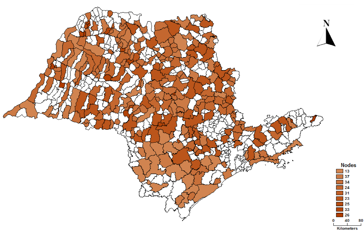
A high predominance of nodes with the highest probability to be critical in the central and upper regions of the state can be observed. The result on the map helps to plan mitigating actions for the municipalities most vulnerable to the occurrence of high mortality rates. It would be possible to have mass actions, such as campaigns due to the proximity between the municipalities of each node.
5. FINAL REMARKS
The Decisión Tree, especially the CART algorithm, made it possible to recognize the main occurrence patterns and variables that most contribute to high and very high fatality rates due to traffic accidents, i.e., the municipality with the highest risk of death by road traffic.
It should be noted that the model aecuracy was not high (61.2%) when compared with models used in other knowledge áreas. However, this value is within the ones found in the literature concerning road safety. It was clear in the extracted classification rules that the highway network extensión, socioeconomic development (represented by GDP) and size of fleet influence the occurrence of high mortality rates due to traffic accidents.
Municipalities with small highway networks, a GDP value around US$7,300 to US$18,700, combined with the truck fleet size are highly likely to have "very high" rates of traffic fatality. Although only 2.2% of municipalities make up this rule, in these cases the rates are twice the worst average rates of the world (WHO, 2015) and must be the first places that deserve special attention from authorities concerning monitoring and planning interventions.
This result is in agreement with other studies that used road traffic accident data to identify association between macroscopic characteristics, such as demographic and socioeconomic data, and a substantial effect on traffic safety, such as crash frequency or fatality (Bougueroua & Carnis, 2016; Lee et al., 2017; Tolón-Becerra et al., 2013).
When the highest probability was "high", most of the rules were related to the size of the vehicle fleet, more specifically, the highest probabilities occurred when the size of the heavy fleet vehicles was médium or large. When the motoreyele fleet was high, the probability of "very high" rates increased, which could be associated to the vulnerability of these users.
Considering that Brazil is a continental sized country that does not have a regular datábase of traffic accidents, this paper has shown an alternative method to traditional models using macro-level data from a datábase that is not specific to traffic accidents to obtain information on common and relevant characteristics related to road safety and to subsidize the actions of the authorities at the macro level.
The approach proposed in this paper could be developed together with the analysis suggested by Figueira, Pitombo, de Oliveira, and Larocca (2017) for áreas where micro-level data are available and, thus, obtain more efficient and completed results, as described by Huang et al. (2016) and Khondakar et al. (2010).
These results are valid for the study área of this paper, once they are limited to only the sociodemographic characteristics of the municipalities. Thus, this rule allows the government to subsidize the planning of actions, characterizing the most critical municipalities for investment in accident prevention, educational campaigns and consequent reduction of fatalities.
Although the number of municipalities classified with very high mortality rates was small, the decisión tree was able to identify them, and indicated relationships between variables that should be better investigated in future studies and that should be monitored. In addition, we also recommend that other studies consider variables related to micro level factors such as crash characteristics, place, weather, time of occurrence, hospital care conditions and characteristics about the victim, for example, as the fatality is influenced by micro and macro level variables.
CONFLICT OF INTEREST
The authors have no conflicts of interest to declare.

