


 text new page (beta)
 English (pdf)
 Article in xml format
 Article references
 Send this article by e-mail
 Cited by SciELO
  Similars in
SciELO
Similars in
SciELO 
 Permalink
1. INTRODUCTION
Flooding in urban catchments involves huge losses to both property and people. The extent of flooding varies from a few streets to complete cities. During monsoon season, due to inadequate facilities for flood management in the drainage system almost all the urbanized cities faces a severe localized waterlogging. Similar issues are also being experienced by many cities in the developed countries because of frequent oceurrences of heavy storms at street level and also due to the poor standard of drains. The condition in developing countries is even more alarming due to the lack of sufficient funds for the expansión and rehabilitation of the existing drainage infrastructure. In developing countries, many large cities experience a high magnitude and frequent flooding which emphasize the need for an improved system that, can be estimated in a conventional drainage modelling approach using available historical flood data.
Some of the severe urban flood events that occurred in recent years are: Chennai (India), 2015 in which 500 people were killed and 18 lakhs people were displaced. This flood was recorded as the costliest flood of the year. In September 2014, Kashmir (India), around 80 percent of Srinagar city was inundated. Around 400 people lost their lives. Dhaka city in Bangladesh usually gets localized flooding events all over the streets during monsoon which hampered the regular activities and traffic in 1996. In the year 1983, heavy storm inundated the Bangkok city (Thailand) for almost six months and caused a property loss of around $146 million (AIT, 1985). The most recent severe flood that occurred in 2016 was in Houston (Texas) which caused huge damage to the property. Due to which the activities in the schools and offices were suspended for a couple of days. This flood had a return period of 15 years. Moreover, New Delhi, capital city of India, due to fast urbanization and rapid migration without simultaneous progress in drainage infrastructure is suffering from serious waterlogging issues which result in loss of property, infrastructure and severe traffic jams. For solving such a big and complex watershed problems, different type of mathematical models are being used by many researchers/designers.
For managing runoff generated in the urban catchments and localized waterlogging issues, several numerical models are available like MOUSE (Danish Hydraulic Institute, 1997), InfoWorks (Wallingford, 2006), HEC-1 (U.S.A.C.E., 1973) and SWMM (EPA Storm Water Management Model) (Rossman, 2010). These one-dimensional (ID) models analyse the complex interaction between precipitation and flooding to genérate an optimum system. There are several studies which have been carried out by different researchers on urban flooding and urban drainage (Gallegos, Schubert & Sanders, 2009: Gires et al., 2012; Holder, Stewart, & Bedient, 2002: Ishikawa, Morikawa, & Iida, 2002; Kolsky, Butler. Cairncross, Blumenthal, & Hosseini, 1999; Posthumus. Rouquette, Morris, Gowing, & Hess, 2010; Rossman, 2010: Schumann, Neal, Masón, & Bates, 2011). The features in these type of models include surface runoff, rainfall, and drainage network's flow routing, water quality, snowmelt and concentration of pollutants (Huber, Dickinson. Barnwell Jr, & Branch, 1998; Martínez, Cansino, López. Barrios, & de la Cruz Acosta, 2016).
In ID hydraulic models, the topography is represented as a series of cross-section in which the model analyse the runoff to evalúate the water level and average velocity at every cross-section. It is a well-organized model with only one limitation i.e. inability of discharge to propágate sideways. The terrain, in a ID model, is represented as a set of cross-sections and not as a surface (Hunter, Bates, Horritt, & Wilson, 2007). Whereas in two-dimensional (2D) hydraulic modelling, the topography is illustrated as incessant surface using meshing technique. Runoff in a 2D model is permitted to flow in longitudinal as well as lateral directions without considering the velocity in upright direction. The lateral stream relationship between the channel and its floodplain can be easily described in this model due to the illustration of terrain as a continuous surface. This makes the 2D model superior to ID model (Schmitt, Schilling, Sasgrov, & Nieschulz, 2002). The only shortcoming is the simulation time which is more than ID model.
Bates, Horritt, and Fewtrell, (2010) reported that 2D models can simúlate water depth and depth-averaged velocity profile more precisely if provided with a correct DEM (digital elevation model), showing clearly the channel and its plain, along with proper inlet and outlet of the channels as the boundary conditions. Few of the 2D hydraulic models used in the past studies are HEC-RAS (2D), DIVAST (Falconer, 1986), LISFLOOD-FP (Bates & De Roo, 2000), JFLOW (Bradbrook, Lañe, Waller, & Bates, 2004), TUFLOW (Phillips, Yu, Thompson, & De Silva, 2005), TRENT (Villanueva & Wright, 2006), MIKE 21 (Carr & Smith, 2007), RiverCAD (Vijay, Sargoankar, & Gupta, 2007), and Nays2DFlood solver (Nelson et al., 2015).
Nays2DFlood (iRIC software) is selected from the above mentioned models for use in the present study. It is one of the recently developed open source models available to analyse the flood flow of any river system. The main advantage of this model is that it requires less number of input variables as compared to other models. The data required are the topography i.e. DEM and inflow at the upstream of each river. Nays2DFlood can be applied to any natural system and it is found to predict reliable results (Wangsa, 2014).
In the present study, iRIC software i.e. Nays2DFlood has been used for the first time to assess the performance of the model and its ability to predict magnitude and extent of the flood in urban catchments. This model is used to simúlate the flow in stormwater drains of Delhi using iRIC and check its suitability in flood application for the urban catchments. This paper can help the administrators in urban planning to mitígate the effects of floods in urban catchments.
2. MATERIALS AND METHODS
2.1 STUDY AREA
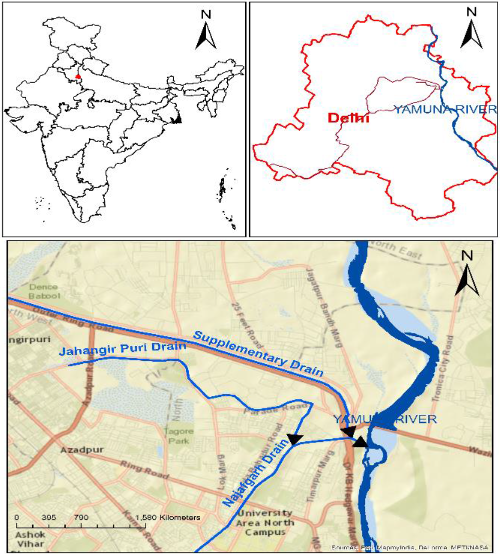
Delhi is situated in the northern part of India and lies between 28°24'17"N - 28°53'00"N and 76°50'24" E -77°20'37" E with an elevation ranging between 213 - 305 m (average elevation 233 m) with respect to the mean sea level (MSL). The study área is a small catchment in Najafgarh basin which comes under the Aravalli mountain ranges in north Delhi. The climate of Delhi has a large variation in temperature between hot summers and cold winters. The temperature varíes from 45°C to 32°C and from 22.2°C to 3.5°C in summer and winter respectively. The humidity is very high during monsoons and very low in summers. The average annual precipitation is 797.3 mm in the city.
In the study área, Jahangirpuri drain, the drain under study, originates just before Azadpur road and carries the surface runoff from the nearby área like Model town, Azadpur, Gopalpur Village and Adarsh Nagar and outfalls into Najafgarh drain at Nehru Vihar as shown in Figure 1. Jahangirpuri drain is a natural stormwater drain which is maintained by Irrigation and Flood Control Department of National Capital Territory (NCT), Delhi. The drain is 5470 m in length and 18 m in bed width having a catchment área of 1619.43 hectares. The catchments área covers the área of Model town, Azadpur and Adarsh Nagar along with a waterbody on the right bank of the drain and Gopalpur Village área on the left bank of the drain.
The major problem in this drain is the back flow which occurs during monsoon seasons. During high storm events, the upstream área gets inundated due to reverse direction flow of the drain resulting in infrastructural and properties loss.
2.2 MODEL DESCRIPTION
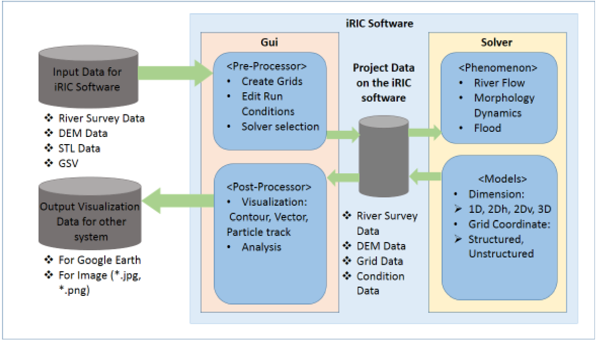
Nays2DFlood is one of the solver available in iRIC (International River Inferface Cooperative) software. This model was first developed by Yasuyuki Shimizu in the year 1990. Later on in the year 2011, the model was integrated in iRIC after the model was further enhanced by Ichiro
Kimura and Toshiki Iwasaka of Hokkaido University. iRIC offers a complete integrated framework where the generic information required by the solvers can be collected, modelling performed and simulated output be analysed. Figure 2, shows the general flowchart of the software procedure. The model solves the Saint-Venant equation which was derived from Navier-Stokes equations (2D) (Cook, 2008). In Cartesian co-ordinate system, the 2D unsteady flow equations i.e. continuity and momentum can be stated as (Jang & Shimizu, 2005; Wongsa, 2014).
Continuity equation:
Momentum equations:
where h = water depth; u, v = depth averaged velocity components; tb = bed shear stress; ρ = water density; H = stage height (H = h + zb); z b , = bed elevation; v = eddy viscosity; t = time; and x, y = spatial coordínate components in the Cartesian system. Components of bed shear stress is as follows:
where Cf = bed friction coefficient; k = Karman constant; and u = shear velocity.
The above equations which was in Cartesian coordínate system, Jacobian chain rules was used to convert it into moving boundary fitted coordinate system. Cubic Interpolation Pseudoparticle (CIP) method, also called the high-order Gudunov scheme, was used for the application of the equation of water flow. The variables are spatially interpolated at the previous time step by using cubic interpolation with the assumption that the spatial gradients were also transported using similar convective equations. Information on a small number of adjacent cells is enough for this approach to compute precise profiles of convectional variables. The changes in the flow and floodplain configuration are numerically computed at the smallest time step allowed by its CFL criterion.
2.3 DATA USED
In iRIC, input data required are DEM (5 x 5 m resolution) and daily discharge rate. DEM used in the present study was procured from the Geospatial Delhi Limited (GSDL), NCT of Delhi. The discharges data was provided by the Irrigation and Flood Control Department, NCT of Delhi.
2.4 MODEL SET UP
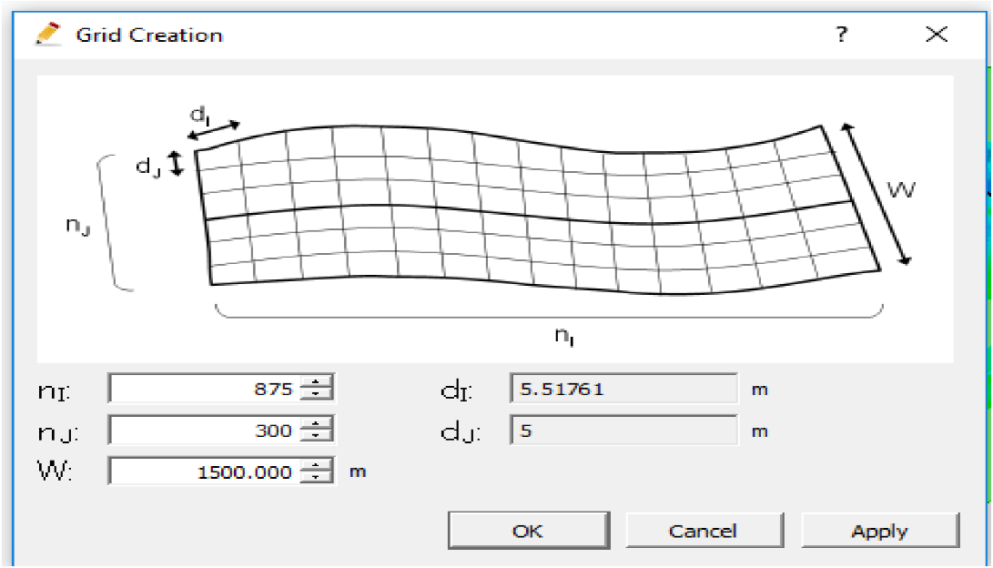
Nays2DFlood solver used DEM/channel cross-section and discharge data to simulate the unsteady flow regime (water depth and flow velocity) . To developed the Nays2DFlood model, first of all elevation data i.e. DEM is imported and then grid is created in longitudinal direction. For creating a grid, first of all grid centreline is set from the upstream to downstream direction.
Then, number of divisions in the longitudinal direction is 875 whereas in the transverse direction is 300. The grid width in the transverse direction is 1500 m. The total grid created is 2,63,676 in numbers with each grid having a size of 5.51m x 5m (di x dj) as shown in Figure 3.
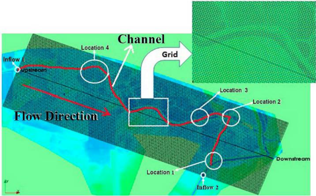
Discharge data was given as inflow 1 and inflow 2 to the model. The inflow 1 is given at the upstream of the Jahangirpuri drain whereas the inflow 2 is given at Bharatnagar Bridge which is located on the Najafgarh drain as shown in Figure 4. The valué of Manning's co-efficient is taken as 0.025 for the urban drains based on the information available in literature. The simulation time steps was fixed at 0.1 sec to avoid the model becoming unstable.
3. RESULTS AND DISCUSSION
A Hydrodynamic model was developed using Nays2DFlood solver which is shown in Figure 4.
The daily discharge data was provided by the Irrigation and flood control department, from the year 2005 to 2013. The highest flood events recorded was for the year 2010 and the highest precipitation recorded was on 20th August, 2010 which was used in the model. Since, our objective is to find out whether the existing drain size is sufficient for extreme events, so the model was simulated and the results obtained was evaluated for the above year.
The Nays2DFlood solver model for Jahangiripuri drain was simulated for 160000sec to understand the occurrence of flooding which includes the two important components namely 1) water depth profiles and 2) velocity profiles.
3.1 WATER DEPTH PROFILE
The water depth profiles for the Jahangirpuri drain is explained as follows.
The flow is normal when it starts from the upstream of the Jahangirpuri drain till location 4. The time required to travel the distance along the drain upto location 4 is 12000sec. After this point at location 1, due to damage bank level and non-uniformity of the drain slope, the runoff starts flowing into the nearby waterbody causing localised flooding as shows in the Figure 5. This is caused because the invert level of the waterbodies is 205.42 m as compared to the drain invert level at 206.1 m. The flow to the waterbodies continúes till the water level of the waterbodies and the level of the drain becomes equal. The máximum runoff observed was 0.38 m. This explain that the cross-section of the drain at this chainage is insufficient to carry the flow of the catchments. The flow then move forward to its outfall but it also continúes to flow towards the waterbodies and inundated the large área as shown in Figure 7.
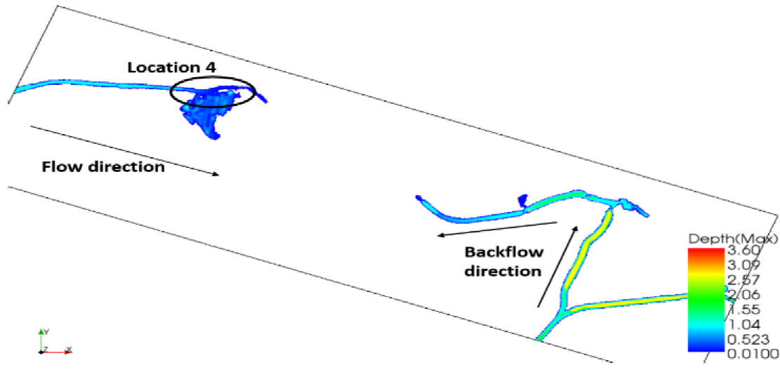
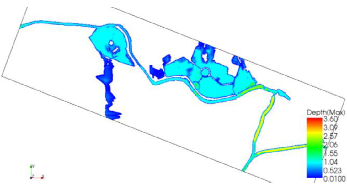
Figure 6, shows that after the simulation of 31000 sec, the upstream flow of the Jahangirpuri drain and backflow coming from Najafgarh drain meets after travelling a distance of 2573 m and 3200 m respectively and at this point from downstream side causing the occurrence of backflow which is caused to the improper gradient of the drain. After that the upstream flow continúes to flow forward towards the outfall and backflow starts mitigating.
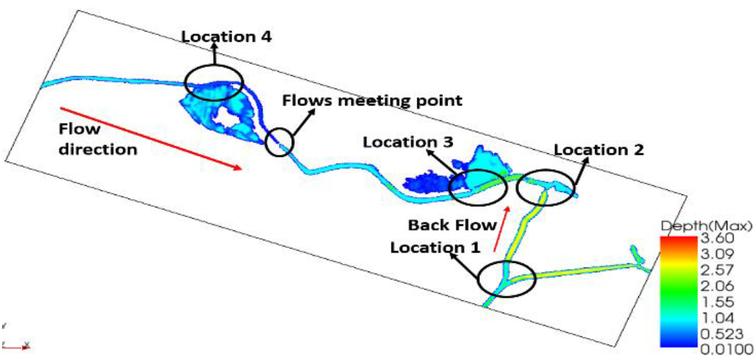
From the Figure 7, after 80000 sec, the máximum water depth at location 3 is 1.57m, at location 2 is 1.54 and at location 1 is 1.55 which are the problematic locations as identified. Although, depth of water level at some segments of the drain shows higher level due to which backflow occurs in the drain. When the water level in the Najafgarh drain increases from 1.57 m to 1.72 m, the flow gets bifúrcate into two directions i.e. one stream flow towards the Najafgarh outfall whereas the other stream flow towards the upstream of Jahangirpuri drain which cause the back flow in the Jahangirpuri drain. The reasons behind this may be improper management of the drain i.e. non uniformity of the slope.
3.2 VELOCITY PRO FILE
Four critical locations (location 1, 2, 3 and 4) were identified from the simulation results at different simulation time.
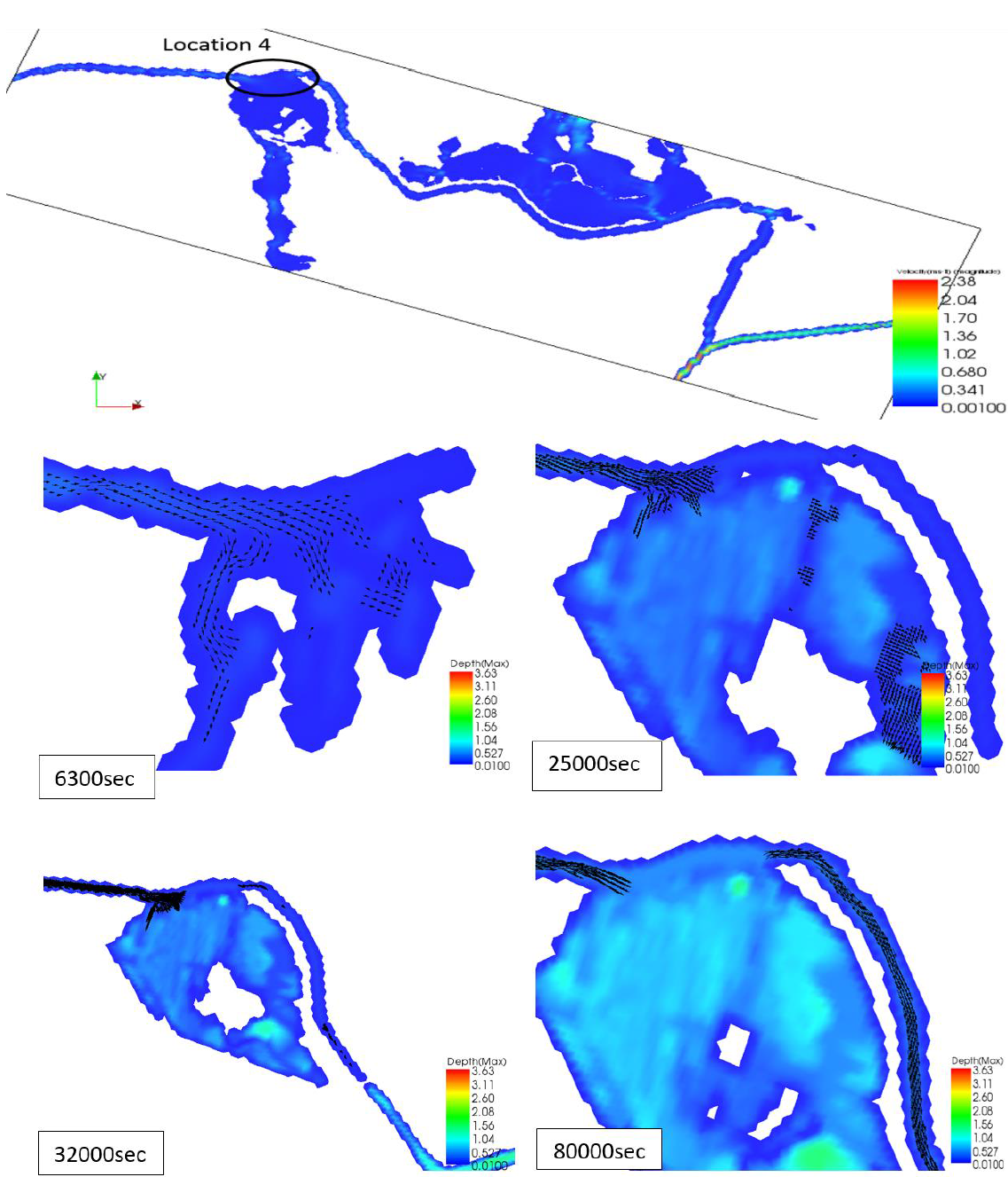
Figure 8, shows the velocity vector profile at location 4. The velocity at the start of the drain is around 0.66 m/sec. But the velocity increases to 0.96 m/sec when the flow reaches location 4. The increase in the velocity is due to the presence of waterbodies at low invert level with respect to the invert level of the drain. The velocity increases due to the sudden drop in the invert level. At 6300 sec, the velocity of flow is 0.96 m/sec when it starts contributing to the waterbodies. At 25000sec, the velocity in the drain reduces to 0.67 m/sec because at this time the level of waterbodies and the level of the drain is almost equal, thus the flow moves forward towards its outfall. The velocity is continuously decreasing over the time i.e. at 32000 sec the velocity is 0.476 m/sec and at 80000sec the velocity is 0.339 m/sec. The decrease in velocity is due to mínimum water level difference as the low level are already filled with water at this time. The flood extent is showing that after inundating the waterbody, the flow moves towards the Model Town and Azadpur área and inundated the complete área. Thus the developed Nay2Dflood solver model can be said as an effective tool for identifying the flood extent during heavy storm events.
The Figure 9, shows the velocity vector diagram at location 3. After this, the velocity is normally low in the drain till location 3. At location 3, the velocity again increases to 1.23 m/sec because at this point all the flow gets diverted to a low-lying área on the left bank of the drain due to sudden fall in the bed levéis. The back water flow of the Najafgarh drain entering into the Jahangirpuri drain with a very high velocity ranging from 2.6 - 3.59 m/sec. The back flow velocity decreases as it travels in the reverse direction up to the of Jahangirpuri drain. Due to the existence of the low-lying área on the left bank side of the drain, the backflow water flows into it. Also due to this backflow, the flow coming from the upstream side do not find the space to flow towards its outfall to contribute to this low-lying área.
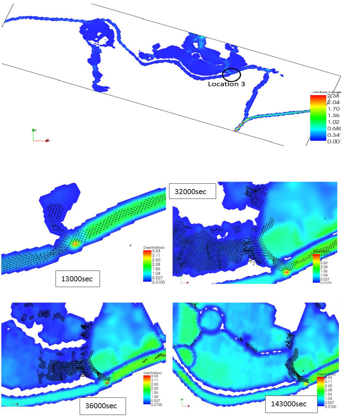
At 13000 sec, the backflow water starts flowing into the low-lying área at a velocity of 1.23 m/sec. After that at 32000 sec, the backflow water velocity is so high that it starts inundating the área at a fast rate as seen in the Figure 8, At 36000 sec simulation time, the upstream flow also starts contributing to this low-lying área at the velocity of 0.33 m/sec. And at 143000sec, the complete área is inundated by the flow and also the velocity get reduced.
Figure 10, shows the velocity vector profile at location 2. At 9000sec simulation time, the velocity is very high 2.75 m/sec. With this velocity the back water flow takes place due to which turbulence is generated in the drain which can be seem from the figure. In this location also, due to poor maintenance of the drain embankment, the flow diverts from the channel and flows into the nearby depression área and the flood the área. At 18000sec, the velocity gets reduces to 1.54 m/sec and the flow becomes almost streamline. Also the flow towards the depression área decreases, as the área is already flood. Again at 32000sec, the velocity increases to 1.66 m/sec due to the vortex formation in the drain. The formation of the vortex in the drain also causes the erosión of the banks due to which sediment deposition takes place. As a result, uniformity of the slope mitigates and reduction in banks cross-section. At 159000sec, the velocity decreases to 1.27 m/sec but the vortex formation in the drain continúes.
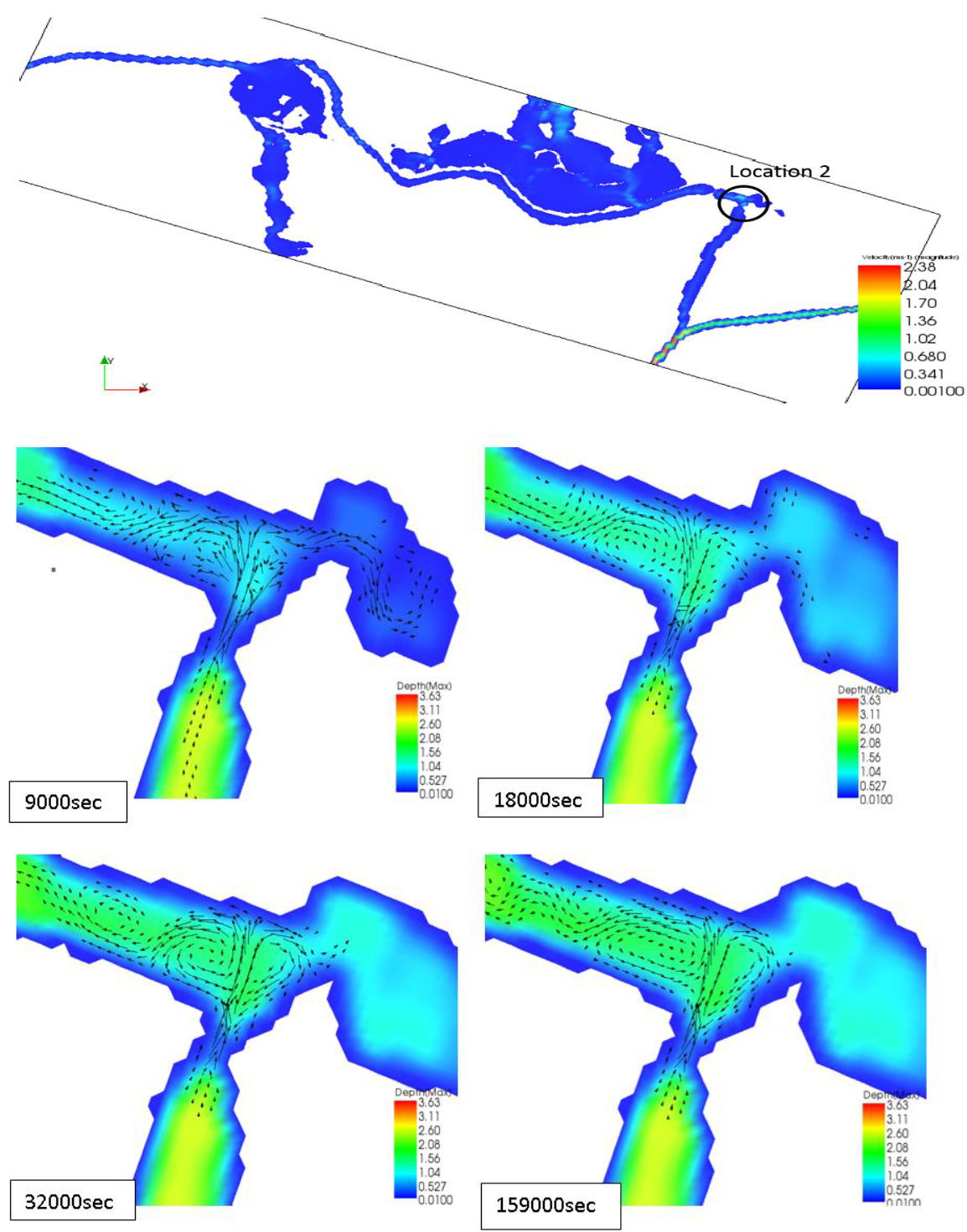
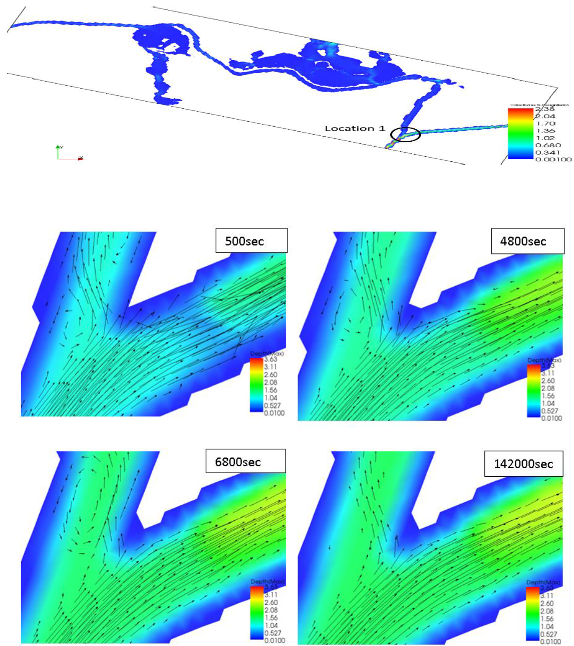
Figure 11, shows the velocity vector diagram at location 1. At this location, the flow from the Najafgarh drain enters into the Jahangirpuri drain and causes backflow problem. At 500sec, the velocity is so high that the backflow into the drain is in the form of zig-zag path. From the figure, it can be seen that the flow is taking place in the curved way due to which the flow along the drain wall will erode the banks sediment and deposition will take place. At 4800sec, the velocity is 1.55 m/sec and initiation of vortex formation can be seen at this location. Complete vortex was formed at 6800sec when the velocity increases to 2.02 m/sec. After that, the backflow was normal till the end of the simulation. The velocity recorded at 142000sec was 1.22 m/sec.
The flooding in this catchments (Azadpur, Model Town and Adarsh Nagar) has been oceurring from many years causing huge losses like property loss, loss of people lives, loss of livestock, etc.
The oceurring of flooding is due to undersize/inadequate drainage infrastructure, siltation which reduces the bed slope. The total flooding área obtained from the simulation is summarized in Table 1.
Tabla 1 Total arca under Flooding.
| S.No | Flooded | Area Flooded (Km2) |
|---|---|---|
| Range | ||
| 1 | 0.011 to 0.527 | 0.4626 |
| 2 | 0.528 to 1.04 | 0.1677 |
| 3 | 1.041 to 1.56 | 0.0574 |
| 4 | 1.561 to 2.08 | 0.0349 |
| 5 | 2.081 to 2.6 | 0.0418 |
| 6 | 2.601 to 3.63 | 0.0002 |
| Total area | 0.7644 |
Since the drain was designed long back ago in the year 1976 according to the available discharge at that time. Over the period, surface runoff has increased exponentially due to urbanisation but no such measure have been taken to manage the excess runoff generated from the catchment. As a result, meandering oceurs in this type of natural stormwater drain and the runoff spill over the bank and flows to the nearby depression and causes localised flooding. The other reasons are the extreme rainfall events. The most important reasons is the improper gradient of drains i.e. invert levéis of the drain is not adequate due to which flow does not able to move towards the outfall and henee, backflow takes place which inundates the area in the upstream.
4. CONCLUSIONS
In this study, a hydrodynamic model was developed to assess the practicability of Nays2DFlood solver as an urban flood simulator in the Jahangirpuri drain, New Delhi, India which experiences large-scale damage during high storm. The model predicted flooding locations which was in cióse agreement with the field observations. In the present study, the model is easily able to identify the critical locations of flooding, backflow. This shows the exaetness of the model behaviour. On the basis of the present study, it has been concluded that:
As the existing Jahangirpuri drain was designed 40 years ago, on the basis of catchment and landuse at that time, the capacity of the drain is inadequate in the present scenario asrunoff has increased drastically because of fast urbanization due to increased population growth. Furthermore, the flood carrying capacities of the stormwater drains have drastically reduced due to excessive sediment load in the drains. Also, sediment accumulation has resulted in adverse longitudinal slope that leads to backflow at location 1, 2 and 3. So, thorough desilting should be done at regular intervals throughout the year, especially before the monsoon seasons, so as to ensure desired slope and depth in the drain.
It has been observed that flood water at location 4 moves to the adjoining waterbody located on the right side of the drain and thus inundated the Model Town and Azadpur area because of the damaged/ improper embankment whereas due to same reason at location 3, the excess flood water breaches the left bank at this location 3 causing heavy floods in Gopalpur Village area. The backwater from the Najafgarh drain makes the flood even worse at location 3. The Model Town, Azadpur and Gopalpur Village area can thus be prevented from such floods by rehabilitating the existing damaged / improper embankment.
As a precautionary measure, pumps of sufficient capacity can be deployed in flood prone áreas. Also, it would be better if no sewage is allowed to flow into the stormwater drain as it not only deteriorates the water quality but also adds heavy sediment load in the drain.
Therefore, based on the model performance in the present study, it can be recommended that the Nays2DFlood model can be effectively applied for simulating urban stormwater drainage systems. Nays2DFlood can be employed to those catchments, where the input information is limited. The model have an addition features like pumps and flap gate modules which can also be used if, present in the field. If the additional input information required by the module are also available, the performance of the model can be improve substantially.

