


 text new page (beta)
 English (pdf)
 Article in xml format
 Article references
 Send this article by e-mail
 Cited by SciELO
  Similars in
SciELO
Similars in
SciELO 
 Permalink
1. Introduction
Maintaining the power system frequency within the permissible limits is an important control task which in normal conditions is carried out by means of load frequency control (Hajiakbari Fini, Yousefi, & Alhelou, 2016; Ketabi & Hajiakbari Fini, 2015a; Kundur, 1994). But, when a sudden power deficit occurs as a result of outage of large generating units or islanding of some parts of power system, even if the existing generating units have enough spinning reserve to supply the demand, their response is not rapid enough to stop the frequency excursion and prevent the operation of generating units protective relays. This may lead to outage of some of the generating units. Consequently, outage of a generating unit can worsen the situation and decrease the frequency to a lower level; therefore, the relays of other generating units might trip and lead to power system blackout. A solution which is widely used in power systems for overcoming this situation is the implementation of under frequency load shedding (UFLS) schemes (Ketabi & Hajiakbari Fini, 2015b; Laghari, Mokhlis, Bakar, & Mohamad, 2013).
In literature, a number of strategies have been implemented for UFLS (Aik, 2006; Anderson & Mirheydar, 1990; Anderson & Mirheydar, 1992; Berdy, 1968; Chuvychin, Gurov, Venkata, & Brown, 1996; Concordia, Fink, & Poullikkas, 1995; Delfino, Massucco, Morini, Scalera, & Silvestro, 2001; Halevi & Kottick, 1993; Hong & Chen, 2012; Hong & Wei, 2010; Larsson, 2005; Lokay & Burtnyk, 1968; Lopes & Mitchell, 2000; Maliszewski, Dunlop, & Wilson, 1971; Pahwa, Scoglio, Das, & Schulz, 2013; Rudez & Mihalic, 2011a, 2011b, 2011c, 2015; Terzija & Koglin, 2002; Thalassinakis & Dialynas, 2004). Conventional method is the first generation of UFLS scheme which has been introduced in (Lokay & Burtnyk, 1968) and developed by some other authors (Aik, 2006; Berdy, 1968; Concordia et al., 1995; Delfino et al., 2001; Halevi & Kottick, 1993; Maliszewski et al., 1971; Thalassinakis & Dialynas, 2004). The first stage in this method is determination of the worst probable generation loss event which results in the highest initial rate of frequency decay. Then, the amount of load shedding which ensures that the frequency will not deviate below the minimum permissible value should be specified. After that, the number and size of load shedding steps are determined based on trial and error to achieve an acceptable operation in case of the worst probable contingency. Determining the worst probable contingency and also the size and number of load shedding steps are not easy tasks. Also, in this method a specified amount of load is shed in every stage without considering the amount of power deficit. Hence, it is probable that overshedding occurs and the frequency increases above the maximum permissible value.
A number of algorithms have been used to optimize the conventional UFLS method (Aik, 2006; Halevi & Kottick, 1993; Hong & Chen, 2012; Hong & Wei, 2010; Lopes & Mitchell, 2000). In Hong and Chen (2012) a UFLS scheme is optimized based on genetic algorithm (GA). To maximize the lowest swing frequency and minimize the amount of shed load, GA is implemented in Hong and Wei (2010). The drawbacks of conventional UFLS can be remedied by using the adaptive UFLS method proposed in Anderson and Mirheydar (1992). In this method, using swing equation, the amount of power deficit is calculated based on the frequency derivative immediately after the disturbance. Therefore, there is no need to determine the worst probable contingency and an amount of load based on the calculated power deficit is shed at the specified stages. In Rudez and Mihalic (2011a, 2011b) the effect of load parameters on adaptive UFLS scheme is investigated. The adaptive UFLS methods estimate the power deficit using swing equation. Hence, these methods are dependent on the equivalent inertia constant of the power system and any change in this parameter may highly affect its performance. Moreover, the estimated power deficit is directly related to the frequency derivative at the moment the disturbance occurs. Therefore, errors in frequency derivative will degrade the reliability of this UFLS scheme.
In Rudez and Mihalic (2011c), a new UFLS scheme based on the minimum frequency of system after disturbance is proposed. As authors claimed, in this scheme no knowledge of power system parameters is needed. In this method, the frequency second derivative is estimated based on Newton method; then, the minimum frequency is forecasted using numerical integration. After that, the amount of load to be shed is determined based on the minimum frequency. However, measuring the frequency second derivative is a challenging problem.
In this paper, a load shedding scheme is proposed in which the frequency of system after occurrence of disturbance is forecasted using the particle swarm optimization (PSO) algorithm. Then, the minimum frequency of system is obtained as described in Section 2. After that, the amount of load which is necessary to be shed to maintain the frequency of system within the permissible limits is determined. Afterwards, the determined amount of the load can be shed in several steps as described in Section 3. In Section 4, requirements for implementing the proposed UFLS method in real power systems have been pointed out. In Section 5, the proposed load shedding scheme is compared with a newly proposed UFLS method through simulation results.
2. Implementing PSO for frequency estimation
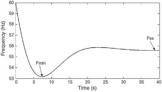
When a disturbance such as generating units outage occurs in a power system and causes a power deficit, frequency drops as shown in Figure 1. This frequency drop can be represented by following equation (Anderson & Mirheydar, 1990):
where
The objective is to forecast the frequency deviation, as precisely and quickly as possible, using the minimum possible measured frequency samples. Hence, for curve fitting, a function should be chosen that represents the frequency of system precisely and has the minimum number of parameters to be estimated by PSO. By trial and error it is found that in the studied power system, the frequency deviation of system up to 3 s after the disturbance can be estimated accurately by fitting a cubic function on frequency deviation samples measured within 0.1 s after occurrence of the power deficit. So, the frequency deviation samples taken within 0.1 s after the beginning of the frequency decay is used by PSO algorithm to determine the parameters of the following cubic function:
As it is shown in Figure 2, frequency deviation of the system up to 3 s after the beginning of the frequency decay is forecasted with a high accuracy. Hence, this data can be used to estimate the frequency deviation of system until reaching the minimum frequency. For this purpose another curve fitting is required. It is found that the frequency deviation of system up to the point of minimum frequency can be estimated accurately by fitting the curve shown in (5) on the frequency deviation data obtained in previous step.

Figure 3 shows that, using the proposed method, the frequency deviation is forecasted with a high precision until the point frequency reaches the minimum value.

To use PSO for obtaining the parameters of above mentioned functions (Δf(t)), it is necessary to determine a suitable objective function to be minimized. In this paper, the following series is selected as the objective function:
Where Δf(i) meas and Δf(i) est are, respectively, the ith sample of measured and estimated frequency deviation and n is the number of frequency deviation samples.
The PSO parameters which are used in this work are given in Table 1. Based on analysis of frequency response of the studied power system, we found that the parameters of (4) and (5) are and located between -5 and 5. Hence, -5, and 5 are assigned v , typical to x min x max , respectively. For c 1, c 2, w, w damp and v max , typical values usually used in solving engineering problems by PSO have been chosen. Max-iteration and N pop have been selected based on trial and error to achieve satisfactory results.
Table 1 Parameters of PSO used for fitting the cubic and main function.
| Parameters | Cubic function | Main function |
|---|---|---|
| c1 and c2 | 2 | 2 |
| x min | -5 | -5 |
| x max | 5 | 5 |
| dx | x max -x min | x max -x min |
| w | 1 | 1 |
| w damp | 0.99 | 0.99 |
| v max | 0.1 × dx | 0.1 × dx |
| Max-iteration | 100 | 100 |
| N pop | 100 | 200 |
Details on PSO algorithm would be found in Eberhart and Kennedy (1995). Also, Pseudo Code for PSO is presented in Van Den Bergh and Engelbrecht (2001).
3. Using the forecasted minimum frequency for load shedding
In the previous section, it was shown that using the proposed method, the minimum frequency would be estimated precisely. In this section, it will be explained how to make use of the forecasted minimum frequency to determine the amount of load to be shed to prevent frequency excursion beyond the permissible limits.
The diagram in Figure 4 shows the relation between the forecasted minimum frequency and the amount of load which is necessary to be shed. In fact, this curve can be implemented to determine the proper amount of load shedding using the forecasted minimum frequency. Then, load shedding is carried out in three or four steps depending on the value of power deficit and after every step, the value of power deficit is estimated for the next step of load shedding using the procedure explained in the previous section. The load shedding process can be summarized as follows:
In the first step of load shedding, an amount of load equal to 30% of forecasted power deficit is shed. After that, the frequency of system until 0.1 s after load shedding is sampled again. Then, the minimum frequency; and therefore; the amount of power deficit are forecasted again. Afterwards, in the second step, an amount of load equal to 30% of forecasted power deficit is shed.
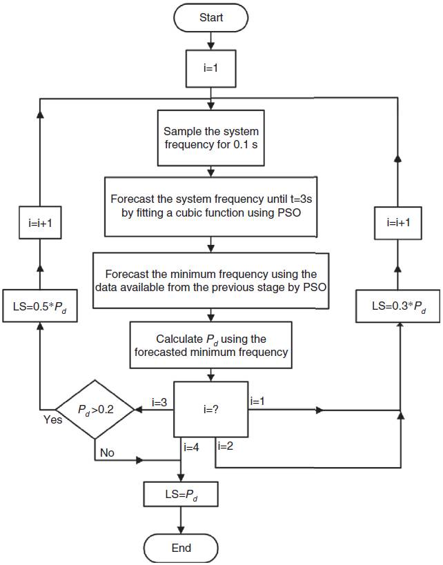
For the third step, if the amount of forecasted power deficit is less than 0.2 P.U., the amount of load shedding will be equal to forecasted power deficit. Otherwise, the shed load in the third step is equal to 50% of forecasted power deficit and the remained power deficit is compensated in the fourth step of load shedding. The flowchart of this load shedding scheme is shown in Figure 5. As simulation results show, for lower values of power deficit the minimum frequency is forecasted with higher accuracy. Therefore, the minimum forecasted frequency of system in every step will be more accurate in comparison with the previous step. So, the minimum frequency will be estimated precisely at the last step of load shedding and shedding the suitable amount of load is guaranteed.

Fig. 4 Adopted load-shedding concept for a particular shedding step, based on the frequency forecast.
4. Requirements for implementing the proposed UFLS scheme in real power systems
To keep the precision of the proposed UFLS method in real world power systems, frequency estimation should be carried out based on a measured frequency with the minimum oscillations. Center of inertia frequency, which is calculated as follows, would be a good candidate for this purpose:
where n is the number of generating units and, f i and H i are the frequency and inertia constant of the ith generating unit.
Frequency of each generating unit would be measured using phasor measurement units and transmitted to the control center to be used in the UFLS scheme. After determining the amount of load to be shed at each stage, based on the load priorities, trip signal is sent to the selected load shedding relays. It is worth mentioning that for transmitting the measured frequencies and trip signals, fast communication links such as optic fiber is required.
5. Simulation results
To carry out studies on frequency stability and load shedding schemes, different models of power system can be used. System frequency response (SFR) model is one of the models widely used for load frequency control and UFLS studies (Aik, 2006; Anderson & Mirheydar, 1990; Chang-Chien, An, Lin, & Lee, 2012; Ketabi & Hajiakbari Fini, 2014, 2015a; Sigrist, Egido, Sanchez-Ubeda, & Rouco, 2010). Due to its simplicity and accuracy, for simulation studies, we have used this model with the typical parameters given in Table 2 (Chang-Chien et al., 2012). Details regarding the SFR model have been presented in (Aik, 2006; Amjady & Fallahi, 2010). It should be mentioned that the aim of the proposed load shedding scheme is to maintain the minimum frequency (f min ) and the steady state frequency (f ss ) above 58.4 and 59.2 Hz, respectively.
The proposed UFLS scheme is tested in case of power deficit ranged from 0.4 to 1 P.U. The results shown in Figure 6 certify that this UFLS scheme responses rapidly to the disturbance and maintains the frequency within permissible limits. For further clarifying, the detailed results of load shedding including the amount of shed load in every step, f min and f ss are given in Table 3.

Fig. 6 The frequency of power system; load shedding scheme is activated due to different amount of power deficit.
Table 3 Detailed results of proposed load shedding scheme.
| Power deficit (P.U.) | Step 2 | Step 2 | Step 3 | Step 4 | Total shed | f min | f ss |
| 0.4 | 0.1099 | 0.0836 | 0.1438 | - | 0.3373 | 59.11 | 59.45 |
| 0.5 | 0.1245 | 0.1137 | 0.1235 | 0.0967 | 0.4584 | 59.27 | 59.63 |
| 0.6 | 0.1370 | 0.1205 | 0.1751 | 0.1257 | 0.5583 | 59.19 | 59.63 |
| 0.7 | 0.1510 | 0.1340 | 0.1749 | 0.1874 | 0.6473 | 58.96 | 59.53 |
| 0.8 | 0.1677 | 0.1384 | 0.2064 | 0.2169 | 0.7294 | 58.73 | 59.38 |
| 0.9 | 0.1850 | 0.1574 | 0.2255 | 0.2913 | 0.8592 | 58.66 | 59.64 |
| 1 | 0.2022 | 0.1706 | 0.2587 | 0.3178 | 0.9493 | 58.5 | 59.55 |
To show the effectiveness of the proposed load shedding method, it is compared with the adaptive load shedding method proposed in Rudez and Mihalic (2011a). For a thorough comparison, several case studies including the impact of power system parameters change on the schemes are carried out. In this paper the ‘adaptive method’ and ‘novel method’ refer to load shedding methods proposed in Rudez and Mihalic (2011a) and this paper, respectively.
5.1. Case 1
In this part, the performance of the two load shedding schemes in case of a power deficit equal to 0.8 P.U. is examined. It is clear from Figure 7 that, in this case, both load shedding schemes can maintain the frequency of system within the allowed limits. The detailed comparative results of both load shedding schemes are given in Table 4.

5.2. Case 2
In adaptive method the power deficit is estimated using the following equation (Ketabi & Hajiakbari Fini, 2015b; Rudez & Mihalic, 2011a):
where, H is the inertia constant of the power system. In this method, the estimated power deficit is directly related to system inertia constant. Therefore, any difference between the value of H used for estimating the power deficit and the real value of H has a direct impact on the amount of calculated power deficit. So, if for any reason, for example an error in estimation of H or variations in inertia constant of system, there is a difference between the value of H used in adaptive load shedding scheme and real value of H, the amount of calculated power deficit will be considerably different from the actual value. Consequently, this will result in malfunction of adaptive load shedding scheme.
In cases which the real 1/H of power system is higher than the value used in the load shedding scheme, the estimated power deficit will be higher than the actual power deficit. But, due to the additional conditions which can cancel some steps of load shedding, the adaptive UFLS scheme will not result in over shedding. It is clear from Figure 8 that both load shedding schemes have a satisfactory performance when the inertia constant of the system decreases. The detailed results of this case study are given in Table 5. From the results presented in this table, it is clear that the proposed method not only results in a smaller amount of load shedding but also smaller frequency deviation.
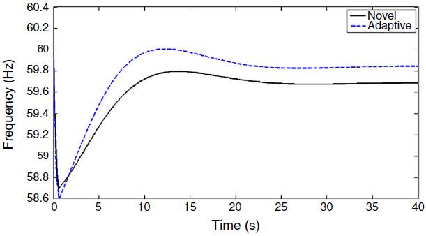
Table 5 Detailed result of novel and adaptive load shedding when the 1/H is increased by 15%.
| Method | Step 1 | Step 2 | Step 3 | Step 4 | Total shed | f min | f ss |
|---|---|---|---|---|---|---|---|
| Novel | 0.1785 | 0.1506 | 0.2139 | 0.2214 | 0.7644 | 58.70 | 59.68 |
| Adaptative | 0.322 | 0.276 | 0.184 | 0 | 0.782 | 58.6 | 59.84 |
However, when 1/H used in the adaptive load shedding scheme is more than the actual value, the calculated power deficit will be less than actual amount of power deficit; therefore; the power deficit will not be fully compensated. Consequently, the frequency of system may decrease to the values lower than allowed limits.
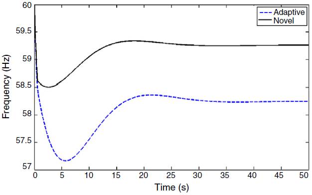
In this case, the impact of decrease in 1/H on the performance of the load shedding schemes is studied. Figure 9 shows that in case of a 10% decrease in 1/H, both of the load shedding methods can maintain the system frequency within the allowed limits. However, as it is shown in Figure 10, decreasing 1/H by 15% the adaptive load shedding method is not successful in preventing the frequency from excursion lower than these limits. The detailed results of performance of both UFLS schemes in these two cases are given in Tables 6 and 7. The results presented in these tables show that by decreasing 1/H, the adaptive method does not shed enough load to maintain the frequency within allowed limits. However, the novel method shows an acceptable performance in this case.


Table 6 Detailed result of novel and adaptive load shedding when the 1/H is decreased by 10%.
| Method | Step 1 | Step 2 | Step 3 | Step 4 | Total shed | f min | f ss |
|---|---|---|---|---|---|---|---|
| Novel | 0.1596 | 0.123 | 0.2119 | 0.248 | 0.7425 | 58.87 | 59.49 |
| Adaptative | 0.252 | 0.216 | 0.144 | 0.108 | 0.72 | 58.39 | 59.29 |
Table 7 Detailed result of novel and adaptive load shedding when the 1/H is decreased by 15%.
| Method | Step 1 | Step 2 | Step 3 | Step 4 | Total shed | f min | f ss |
|---|---|---|---|---|---|---|---|
| Novel | 0.1558 | 0.1391 | 0.1712 | 0.2826 | 0.7487 | 58.94 | 59.55 |
| Adaptative | 0.238 | 0.204 | 0.136 | 0.102 | 0.680 | 58.15 | 59.94 |
This case study shows that the novel load shedding method is not sensitive to changes in inertia constant of power system and has an acceptable performance in this case.
5.3. Case 3
It is probable that generator outage occurs during the load shedding process as a result of a fault or malfunction of generators underfrequency relays. This will result in an additional power deficit during the load shedding process. So, for maintaining the stability of power system, it is necessary for the load shedding schemes to consider this additional power deficit in the next steps of load shedding.
In this case study, the performance of both of the load shedding schemes in case of an additional 0.2 P.U. power deficit, 0.3 s after the initial 0.8 P.U. power deficit, is investigated. The adaptive load shedding method calculates the power deficit just after occurrence of the initial power deficit; so, it is not able to recognize the additional power deficit. Consequently, the additional power deficit is not compensated by the adaptive UFLS method and as Figure 11 shows, this results in excursion of frequency out of the permissible limits. But, the novel scheme, estimates the power deficit after every load shedding step. Therefore, it is able to recognize the additional power deficit and consider it in the next load shedding steps. Figure 11 certifies the proper performance of the novel UFLS scheme in case of additional power deficit during the load shedding process.
6. Conclusion
A novel load shedding method, based on forecasting the minimum frequency, is presented in this paper. It is shown that by using the proposed method, the minimum frequency is estimated with a high precision. Therefore, the power deficit can be estimated precisely; then, the proper value of load can be shed at the proper time. Based on simulation studies, the proposed UFLS scheme has been compared with one of newly proposed methods. Superiority of the proposed method in different case studies has been confirmed. It has been demonstrated that, in cases where parameters of system are not changed, the proposed method sheds less load and also results in a smaller frequency deviation. In addition, simulation results verify that the proposed load shedding scheme is independent of power system parameters and even in case of system parameter variation, it is able to keep the frequency within the allowed limits. Furthermore, it is proved that this method has a proper performance when an additional power deficit occurs due to outage of generating units during the load shedding process.

