1. Introduction

In order to fulfill capital requirements needed in Advanced Measure Models defined by Basilea II agreements, financial institutions must use internal data, relevant external information, scenario analysis and factors so that firms business environment as well as its internal control system improves. Up to now internal historic data of operational risk losses have been insufficient to predict future, furthermore, there is not sufficient information to estimate frequency and severity of losses in a safe way (^{Chen, et al., 2013}). On the other hand, external data are difficult to obtain due to operational treatment diversity among financial institutions (^{Zhou et al., 2014}). Examining causes and effects of losses is relevant when an Operational Risk Analysis is executed.

Scenario analysis can be subjective by itself; however combined with historical data of operational risk losses it turns into a powerful tool for estimating this type of risk. There are crucial aspects regarding operational risk management that can be explored by cause-effect models (^{Chonawee, et al., 2006}). Bayesian inference has proved to be a worthy technique for combining incomplete data with expert opinions.

Operational Risk (OR) is defined as potential loss because of fails or deficiencies in internal controls, errors in processing and loading operations or information transmission, as well +by adverse administrative and judicial resolutions, frauds, robbery, technological and legal risk (^{CUB, 2005}). This definition includes operational and legal risk but excludes reputational risk. OR is classified as a quantifiable and non-discretionary risk because it cannot be generated due to taking risk positions.

OR is the eldest of all risks a financial institution might confront, in general is inherent to all activities where people, process and technological platforms intervene in, and so is not exclusive of financial activities.

Basilea II document (^{BIS, 2005}) denotes that in order to qualify for operational risk of capital measurement by an Advanced Measure Models (AMM) institutions have to prove internal modeling precision, for each entry of the risk matrix created on eight business lines and seven relevant risks types. If institutions want to achieve regulatory requirements, modeling must embrace:

There are several more aspects while modeling operational risk according to ^{Chavez et al. (2006)} and ^{Cruz (2004)}, if a Loss Distribution Approach (LDA) model is used, then financial institutions must quantify frequency distributions and severity of operational losses in each entry of the risk matrix within a year time interval. Regarding OR, there are some applied approaches that estimate OpVar using several different methods, see ^{Venegas-Martinez (2006)}, ^{Martinez-Sanchez and Venegas-Martinez (2013a}, ^2013b, ^2013c).

Main objective of the present research is to quantifying capital requirements of OR based on Bayesian inference by using an operational risk advanced measurement model, particularly when historical information is not available for a typical Mexican financial institution. The model employs a conjugated Poisson-Gamma distribution and feeds from experts interviews information so parameters can be measured. It is expected a direct and positive relationship between unexpected events and economic losses.

This document is organized as follows: an annual loss model thru business line and event type for estimating operational risk is presented in section 2, Bayesian inference theory is explored in section 3, a Bayesian analysis with a conjugated Poisson-Gamma distribution for estimating frequency and severity in a financial firm is performed in section 4, operational risk capital is estimated by using the parameters obtained from Bayesian analysis in section 5, main conclusions are characterized in section 6.

2. Annual Loss Model

A model with a single risk entry (business line/risk type) for annual losses is a process compound by:

where n is the number of annual events modeled as a random variable with a discrete Poisson distribution and P_i = 1, 2,…n are the severity of the events modeled as an independent random variable of a continuous distribution. Frequencies n and severities P _i are assumed to be independent conditions of parameters distribution. Estimation of +annual loss distribution modeling frequency and severity is a typical technique (^{Klugman, et al., 2012}).

Frequency and severity estimation is a challenge specially because OR main characteristics when low frequency and high impact events occur, more so if insufficiency or scarcity of historical data exists. Among institutions external information sources are hard to find and even harder to apply because of the operations volume and the individual operational characteristics of them. Therefore, is complex to estimate probability distributions using only internal and external data, in fact information available presents limited capacity of predicting the future due to uncertainty environments, if information exists.

Hence, is very important to incorporate scenario analysis in the model since financial institutions use it to identify risks, so internal and external expertise of events can be found, current controls as well as those to be implemented in the future can be identified, etc. Moreover, is possible to recognize weakness, strengths and other factors acquired through an approximated quantitative evaluation of frequency and severity distributions based on experts knowledge; subsequently this type of analysis must be combined with LDA models.

Bayesian inference is a technique that integrates experts knowledge and data analysis (^{Buhlmann and Gisler, 2005}). This method creates structural models where experts knowledge is incorporated by specifying a priori distributions of models parameters, which are updated as information becomes available. At any time an expert can evaluate the a priori distribution based on new information and to include it into model. In the following section, Bayesian inference technique is described in the context of OR and is implemented in the quantification of OR for a financial institution. For the purpose of the present research, an expert is defined as an extremely experienced official employee with knowledge in operation and vulnerabilities of financial institutions.

3. Bayesian Inference

Bayesian approach is based on the subjective interpretation of probability, as a degree of believes respect uncertainty, see ^{Venegas-Martinez (2008, Chapter 73)}. Bayesian inference considers an unknown parameter as a characteristic where a degree of believes can be expressed from and also be modified because sample information. A parameter is a random variable with an a priori distribution based on a probability assigned before sample evidence, when evidence is gotten the a priori distribution is adapted so a posteriori distributions emerges and inference respect the parameter can be formulated.

If a random vector of observations P = (P₁, P₂,…, P_n) with a density of h(P | θ) for a vector of parameters θ = (θ₁, θ₂,..., θ_k) is considered, where observations and parameters are always weighted as random ones, then Bayes theorem can be expressed as:

where π(θ) is the parameters density also known as a priori distribution, π^ (θ|P) is the parameters density given by observed data P, also known as a posteriori distribution, h(P, θ) is the jointly density of observed data and parameters, h(P | θ) is the density of observations given by parameters and h(P) is the marginal density of P. If π(θ) has a continuous distribution, then marginal density can be written as:

For the case of discrete distribution,

For simplicity in notation π(θ) will be considered only in a continuous way. The objective is to estimate predictive distributions of frequency and severity for each observation P_n+1 given the available information P = (P₁, P₂,…, P_n). If parameters θ, P_n+1 and P are pairwise and mutually independent, then conditional density given the vector of observations is:

By assuming that P = (P₁, P₂,…, P_n) and P_n+1 are identically and independently distributed given 9, then using equation (2) the following a posteriori distribution is gotten:

where h(P | θ) is the probability function of observations, h(P) is a normalization constant from which a posteriori distribution function can be seen as an output of "previous knowledge" because observations of probability function. Since scarcity of data is a relevant scenario for studding OR it is proposed that:

Bayesian estimations approach leads to optimum estimations that minimized the quadratic error of prediction (^{Buhlmann and Gisler, 2005}).

4. Bayesian Analysis

Conjugated distributions are useful when Bayesian inference takes place. If F denotes a variety of density functions ƒ (P | θ), indexed by θ, and one kind U of an a priori set of densities π(θ) exists, then π(θ) is a conjugated family for F if the a posteriori density is f (P) = ∫f(P|θ) π (θ) dθ, and is part of the kind UⱯƒ ∈ F and also π ∈ U. If a complete family U contains all distribution functions then is a conjugated family of F as well, nonetheless it is important that U be as small as possible meanwhile keeps a realistic distribution.

Conjugated pairs of functions F - U more engaged for modeling frequency and severity in an OR analyses are: Poisson-Gamma, LogNormal-Normal and Pareto-Gamma (Anghelache, Olteanu, 2011). In all these cases a priori and a posteriori distributions are the same kind, hence a posterior distribution parameters are easy to calculate by using a priori distribution parameters and observations. In this analysis a Poisson distribution is employed for modeling frequency when unexpected events could generate an extremely economic lost, that is severity, which is modeled by a Gamma distribution. Therefore the use of a conjugated Poisson-Gamma distribution is in order to estimate OR.

Poisson distribution is one of the most used function distributions in OR modeling of losses frequency where occurrence frequency is not constant over time. Consider N = (N₁ , N ₂,…, N_n) number of observations for a independent random variable with a Poisson distribution (λ) and conditional density that stands for the number of OR events observed within the financial institution, with a log likelihood given by:

and the a priori distribution for A is a Gamma distribution (a, f) with a density function given by:

If λ and N₁, N₂,…, N_n are independently as well as known, then the probability function is:

By using equation (6), the a posteriori distribution is:

Consider now,

The a posteriori distribution function is a Gamma α^,β^ distribution as the same as the a priori distribution but with parameters α^,β^. The expected number of events, given by observed data, E (N_n+1|N) will be the a posteriori distribution measure as,

The more the number of observations n is, the higher the value of w will be giving a higher weigh to observations and a lower weigh to experts opinion; the less the number of observations, w decreases and the experts opinion has a higher weigh. In order to incorporate updated data, the same process must be carried out in a recursive condition. Considering observed events N ₁ , N₂,…, N_k and assuming an a priori probability distribution π (λ|α, β), the Gamma (α, β) function is initiated and the a posteriori distribution function π^λN1, N2, …, Nk after the k observation is the Gamma distribution α^k, β^k with:

where,

Thus allows a posteriori distribution parameters to be based on recently observations and be calculated by updated data as becomes available. Experts can estimate the number of events, λ, but will not have absolute certainty of their estimation. The best approximation will be E [E (N| λ)] = E (λ). If the expert specifies E(λ) and has the certainty for a true value of λ to be within the interval (a, b), with probability P [a ≤ λ ≤ b] = p, then parameters α and β can be estimated numerically.

The accumulative Gamma α, β distribution function is:

So α and β are easily estimated. Now lets consider the information from a financial institution where experts deliberate that E (λ) = 1.2 and P [0.8 ≤ λ ≤ 1.5] = 0.70, so the a priori distribution will be a Gamma (a ≈ 11.8273, β ≈ 0.1015).¹ If we assume that the financial institution will face 2 losses within a year once the a priori distribution has been estimated, then by using equation (16) the a posteriori distribution parameters are:

If in the following year a loss is observed, then the a posteriori distribution parameters will be:

and

With further observations λ^ value will be updated as equation (16) shows. Therefore, observed data will update the distributions for events with an initial condition based on an experts opinion.

5. Capital Risk Measurement

The financial institution has no constrain regarding any regulations to specify the confidence percentage that loss distribution must be estimated at; since the Comision Nacional Bancaria y de Valores of Mexico does not stipulate a specific value on its regulations, the financial institution decided it should be 95%. Assuming frequency has a distribution P (.|λ) and severity is measured by ƒ (.|α), given A and a, also a posteriori distribution function π^λN and π^αX where are λ and α estimated thru distribution functions defined by experts, the loss distribution can be calculated using Monte Carlo method as follows:

Since there is scarcity of data for calculating OR capital, Bayesian net has to be updated as soon as new information comes up form risk events. The expected number of risk events (N) for the firm is 1.20 and expected loss severity (X) is $2,300.00 pesos. Under independency,

In order to calculate a loss distribution by Monte Carlo method, Poisson frequency distribution is assumed with λ =1.20 and Gamma distribution with (α ≈ 11.8273, β ≈ 0.1015), and then:

The OpVar at 95% confidence level gives a maximum expected loss of %18,297.00 pesos from which expected loss is $2,760.00 and a non-expected loss of $15,537.00 pesos. The latter estimation was conducted by selecting λ =1.2 while P [0.8 ≤ λ ≤ 1.5] = 0.70, which is the average value for the Poisson distribution. In order to see how the OpVar behaves within the entire interval, the whole simulation process described previously was repeated for 6 different combinations of values of α, β and λ, the results are summarized in Table 1, by setting λ = { λ | λ ∈ R, 0.8 < λ < 1.5} since corner values produce no plausible Gamma distribution parameters. Table 1 shows all simulations.

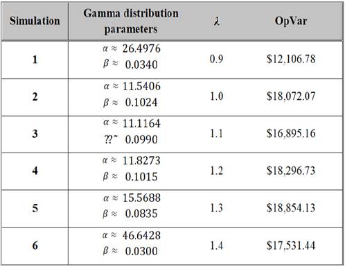
It is easy to see that OpVar increases as Poisson distribution parameter does it as well, in fact there is a positive correlation between them since ρ_λ,_։o_pv_ar = 0.185514, thus been consistent with the theory. The corresponding losses values for the set of simulations are presented in Graphic 2 where it can be analyzed severity and frequency as well. In all simulations a small loss value, around $3,000.00 pesos, present a high frequency among the 10,000 observations, then as losses values are getting higher frequency starts to decline until OpVar is reached, afterwards frequency and severity jointly decline. Most frequency distributions are bimodal shaped.

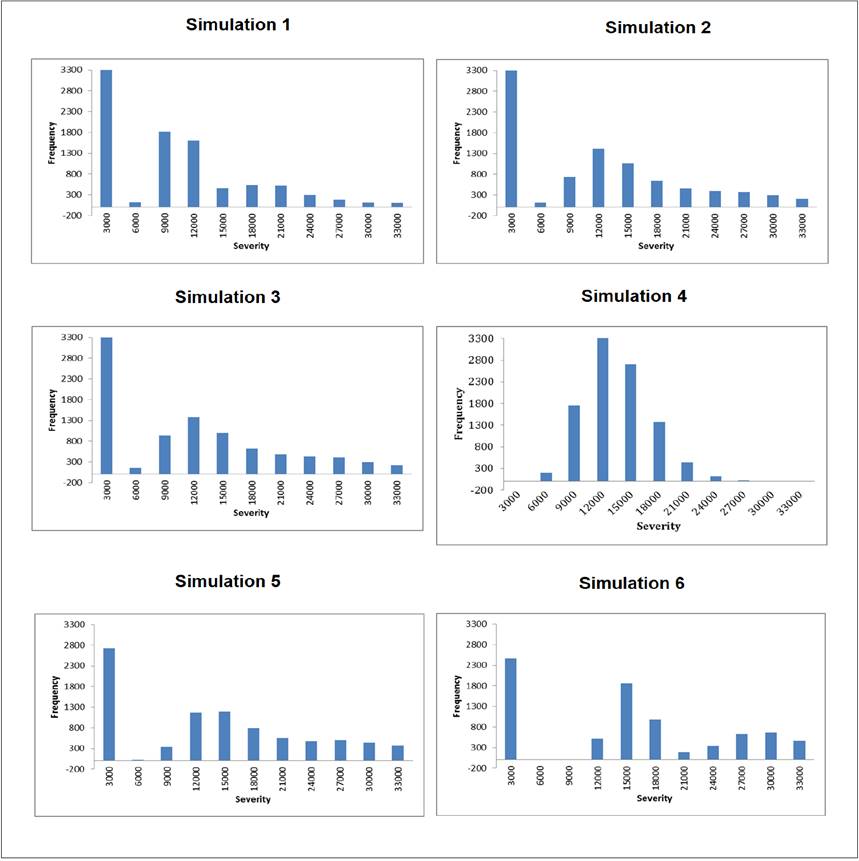
OR is characterized by the occurrence of low probability events with elevated severity, this kind of events rarely happen so there is not enough information available within financial institutions or statistically significance data bases that can be used to perform goodness-of-fit tests; most of this tests are based on the measurement of the distance between observed and estimated data. Nevertheless the above graphics show an acceptable distribution fit.

Also it is important to highlight that since knowing the economic impact as real as possible is desirable, a Monte Carlo without variance reduction must be used. Monte Carlo simulations with variance reduction generate biased values, hence biased distributions.

On the other hand, when the expected number of events takes values from 0.9 to 1.4 then expected OpVar is $16,959.39 pesos with a volatility of $2,469.64 pesos, therefore OpVar dynamics can be easily shaped, see Graphic 3.

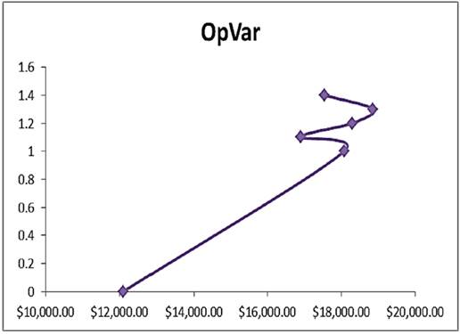
As long as experts expected event increases, OpVar will increase as well. Even more, OpVar is bearable when only one losses event occurs nevertheless OpVar gets higher each time losses event occurs, it is important to highlight that OpVar tends to increase for integer values. As long as unexpected events occur twice a year at most, economic lost will be bounded $16,000 and $18,000 pesos. Consequently it is necessary for the firm to design a strategy to avoid losses events.

6. Conclusions

Through Bayesian inference theory the present research quantifies frequency and severity of Operational Risk. This method is based on parameters specifications from experts for an a priori distribution of frequency and severity distribution functions by using available data of a financial firm. Afterwards, observed data and parameters for a posteriori distribution estimations are weighted so OR capital is calculated for a year time line. Calculations are simple and one mayor advantage of this method relays in jointly considering experts knowledge and historical data for a financial firm, thus allows determining operational risk capital thru internal data. Furthermore, the model can be updated and calibrated as soon as new information comes up during financial firms operations, which will give more reliability and strength to modeling operational risk, and hence to inference collect from it as well. For a set of simulations it can be proved that a positive relation between OpVar and experts event values exists and that frequency and severity of losses is directly related to OpVar optimum value at 95% of confidence. Consequently, this research provides with an empirical model that uses prior information usually delivered by experts within financial institutions so operational risk can be managed.

Main advantages of using Bayesian inference to calculate low frequency risks such as operational risk events, consist in getting stable values due to combining experts opinion and few available data along with the proposed methodology, also in specifying an apriority distribution so frequency and severity can be estimated simultaneously, in weighting the a priori distribution with current data to estimate a posteriori distribution in order to obtain new model parameters.

Finally, we can calibrate the network by incorporating new event information as it is obtained over time. It is important to note that the OpVar can be easily measured with little information even with one or two observations, so there is no dependence on a huge set of information. One disadvantage is that an experts opinion can be untrusted, so is recommendable the expert to be part of the core staff in the financial institution.