


 text new page (beta)
 English (pdf)
 Article in xml format
 Article references
 Send this article by e-mail
 Cited by SciELO
  Similars in
SciELO
Similars in
SciELO 
 Permalink
1. Introduction
One of the certainties in the global financial industry refers to the explosive growth in trading amounts from commodities, either due to the needs of the real economy or the exponential increase in derivatives positions (leveraged or unleveraged). These facts, alongside the intrinsic characteristics of commodities, namely the high correlation with climate factors and the oligopolistic nature of these markets contributed to incite an upsurge in volatility levels that ought to be tackled with a view to preserving the financial health of the banks.
Back in 2006, the BCBS rapidly acknowledged the volatile nature of these markets and enacted a three-pronged regulatory framework composed of two standardised appraisals: Simplified Approach and Maturity Ladder Approach on the one side and the usual model-derived VaR-based Internal Model, although it maintained the typical ambiguity at the time of indicating the avenue to ascribe to and furthermore, remained agnostic as to circumscribe the IM to any adequate methodology. As far as directives for commodities are concerned, Basel II contained one distinctive element that differed from other kind of exposures, most importantly stocks: instead of limiting the SA to the widespread 8%, the rate was fixed at 18%, thus paying heed to the instability of commodity quotations. However, even though the appraisal could appear more adequate than their fellow regulated markets, the BCBS decided to alter the tack in the wake of the subprime crisis of 2008.
According to the first post-crisis Banking Banana Skins issued in 2014, more than 650 respondents from all over the world expressed that the greatest threat to the banking industry lies in the strong regulatory and political back- lash that has taken place against banks in reaction to the crisis. Furthermore, these risks were ranked first and second respectively out of a field of 28 risks in the survey (CSFI and PwC (2014) ). Hence, participants in the financial arena overwhelmingly fear that the weight of the new regulation is becoming excessive, to the extent of potentially damaging banks and halt the economic recovery. These conclusions automatically direct the attention towards Basel III which, in many respects, cracked down on several aspects of market risk measurement, thus giving birth to several misalignments referred to the right incentives to apply the most appropriate techniques and policies.
The present paper explores in detail the topics connected with the inter- play between the SA and the IM, with the supporting VaR computed through different techniques, and its close relationship with the issue of the motivations that hover in the background. In this sense, the research highlights a host of regulatory implications: i) highly leptokurtic schemes reveal themselves as the most precise to deal with abnormal adverse market movements; ii) models re- lying on Extreme Value Theory perform most consistently, delivering extensive coverage; iii) unlike the exercise for stocks, the 87.50% increase in the SA's flat rate renders it relatively sharp for MCR purposes; iv) the mere existence of an (adequate) SA dampens the lure of the most precise conditional volatility models (i.e., EVT); v) providing sharp models were implemented, Basel II framework would have more than enough served its intended purpose, thus rendering Basel III provisions absolutely disproportionate; vi) huge disincentives to apply accurate models surge, which could be softened by diminishing the fixed multiplication factor mc and mc and ms under Basel II and Basel III respectively, in order to equate the performance of IM and SA approaches.
The article unravels as follows. Chapter 2 briefly reviews some patterns about commodity essential for the text; Chapter 3 states the Basel regulatory structure for commodity risks; Chapter 4 provides the Methodology; Chapter 5 analyses the data at hand; Chapterss 6 and 7 describe the exercise utilising Basel II and Basel III configurations, whereas Chapter 8 scrutinises the question of the moral hazard and the right enticement to use accurate models for MCR determination in association with the security in times of colossal crises. Finally, Chapter 9 reflects on the whole process.
2. Few Facts about Commodity Markets
Trading in commodities represents an important proportion in today's market transactions. In effect, the volumes traded under this concept have increased significantly in the last decade: the January 2014 Outlook recently released by the World Bank (World Bank (2014)) reveals that the funds traded around the world have augmented from 38.1 in the first quarter of 2001 to 325.8 in the third quarter of 2013 (both measured in billions USD), which amount to a staggering 750.65% (Graph 1).That upward trend appears to reflect a threefold effect: increased demand (particularly as a result of the economic boom in China), limited supply (due to a variety of reasons, principally meteorological) and, thirdly, increased prices as a natural consequence of the first one, although Algieri (2012) identifies some degree of speculation and excessive speculation behind those somewhat extreme price movements.
It is often the case that those abrupt jerks in values crystallise in high volatility levels which, by the way, is the main reason that attracts speculators (Geyser and Cutts (2007)). High volatility is, then, a typical feature of commodity markets, fostered by the structural tendency to abrupt fluctuations due to the short-term inelasticities of supply and demand for agricultural products and metals (Cohen (1999)), politically induced variations in stocks for energy materials and income-driven demand for precious metals. According to the World Bank (2013), the rising price volatility is inscribed in commodity supercycles which have been taking place more or less regularly since the 19 th century.
All things considered, small swings in supply and demand patterns may exert considerable effects on market prices, thus enhancing volatility (Valenzuela, Martin and Anderson (2006)). It is noteworthy that, owing to their nature, commodity prices move in cycles and, furthermore, tend to record ap- proximate conjoint displacements. In line with the topics to be dealt with, the aforementioned facts can be appreciated resorting to three series of monthly indices retrieved from the World Bank website: agriculture, energy and precious metals. Graph 2 and Chart 1, which depict the behaviour of these series in the period 1976-2007 reveal the same characteristics present in almost every financial security series 1 (Alexander (2008b), Christoffersen (2003), Penza and Bansal (2001)): absence of drift, asymmetry (positive) and leptokurtosis although the most remarkable feature is given by the abnormally high volatility (measured by the standard deviation of the log-returns) values: 6.54%, 2.32% and 5.52% recorded for energy, agriculture and precious metals respectively, due to an array of factors likely to be subsumed by disturbances in supply and demand (courtesy, in turn, of climate and macroeconomic imbalances).

Graphic 2: Agricultural, Energy and Precious Metals series 1976-2007 Monthly indices based on nominal USD, 2010=100
Additionally, McKinsey (2013) emphasises the cyclical behaviour of commodity prices, localising at least three commodity supercycles since the 19 th century, besides the one beginning in the late 1990s. Incidentally, the dashed vertical line in Graph 2 signals Jan-1999 as a period of huge price increases that up to Dec-2007 delivered 497%, 67% and 179% for energy, agriculture and precious metals respectively. However, as a consequence of the financial crisis unravelled in 2008, the trend somewhat reversed and the values for the same indices fell 45%, 19% and 15% respectively.
Finally, co-movements across commodities constitute a relevant pattern not to be neglected at the time of elaborating regulations or building portfolios. In effect, Chart 2 -Panels A and B -, deploy the correlation coefficients between the energy, agriculture and precious metals monthly indices: Panel A, featuring the period 1997-2007, points to correlation coefficients in the region of 12% (energy-agriculture), 22% (energy-precious metals) and 29% (agriculture- precious metals), whereas in Panel B, dealing with year 2008, the coefficients swell dramatically: 84%, 39% and 65%.


The above examples constitute only a token of the main characteristics of commodity series. Bearing in mind that commodity prices have historically been among the most volatile of international prices (even exceeding that of stocks, exchange and interest rates) and frequently exhibit abrupt jumps and steep falls, many difficulties arise at the time of determining underlying distribution of prices and trends in prices (Kroner, Kneafsey and Claessens (1993)). These uncertainties, in turn, are susceptible of springing up when policy makers draft regulations regarding the impact that positions on commodities should exert on the financial health of a bank.
3. Basel Regulatory Framework about Commodities Risk
3.1. Basel II Structure
Prior to eliciting the treatment dispensed to commodities risk, it is important to state that the Basel Committee (BCBS) defines commodity as "a physical product which is or can be traded on a secondary market, e.g., agricultural products, minerals (including oil) and precious metals" (BCBS (2006: 182)). However, it explicitly excludes gold, which is classified as a foreign currency and, consequently, regulated under those guidelines.
The Basel Committee acknowledged the risk posed by commodities early in the Basel II Capital Accord, stating clearly that "The price risk in commodities is often more complex and more volatile than that associated with currencies and interest rates. Commodity markets may also be less liquid than those for interest rates and currencies and, as a result changes in supply and demand can have a more dramatic effect on price and volatility. These market characteristics can make price transparency and the effective hedging of commodities risk more difficult." (BCBS (2006: 182)). The BCBS asseverates that commodities risk arises from four different sources:
Directional risk: risk of change in the spot price of the respective asset arising from net positions. This variety corresponds to spot or physical trading which, were the institution to be engaged in portfolio management strategies including derivative contracts, would be accompanied by: 2
Basis risk: risk of variation in the relationship between prices of similar (not identical) commodities;
Interest rate risk: risk of change in the cost of carry for forward positions or options;
Forward gap risk: risk of modifications in the price of forward positions for every reason but interest rates. It is noteworthy that risks c) and d) grasp the risk from mismatches in the maturity of derivatives positions.
In order to tackle the former perils, the BCBS sticks to a dual structure comprised by a deterministic approach and a more risk-oriented model-based one featuring a risk metric, i.e., Value-at-Risk. Therefore, a three pronged strategy is set out: a) Maturity Ladder Approach (MLA), b) Simplified Approach (SA) and c) Models Approach (MA). Banks are allowed to select the most convenient methodology provided it covers the four risks mentioned. In what follows, a succinct explanation of the three appraisals is provided.
3.1.1. Maturity Ladder Approach
The MLA distinguishes between Directional risk, on the one hand, and Basis, Interest rate and Forward gap risks on the other. For the last three risks, the BCBS contemplates the allocation of all the net commodity positions according their maturity into a time-ladder which, in the end, increases the sum of the long and short positions matched (called gross position) by 1.5%. Any residual position may be carried forward to balance more prolonged exposures. However, acknowledging the imprecision of the matching (hedging) mechanism among different time-bands situated further out, an extra charge of 0.6% of the net position carried forward is to be added wrt every interval that the net position is brought forward. At the end of the process, a capital charge of 15% must be applied, thus accounting for Directional risks.
3.1.2. Simplified Approach
The SA bears much resemblance to the Standardised Approach applied in the case of stocks, though in view of the volatile characteristics of these markets the rates are fixed at a higher level. Like the MLA, the BCBS distinguishes between Basis, Interest rate and forward gap risks on the one side, and Directional risks on the other. The present appraisal could be regarded as a limited or restricted MLA given that it precludes a 3% surcharge for the first group of risks and a 15% for the second. Consequently, the capital charger presents at least an 87.50% increase vis-a-vis the Standardised Approach envisaged for stocks.
3.1.3. Models Approach
The achievement of MA roots in the opportunity to determine the market risk MCR based on VaR estimates derived from own models. MCR result from:
i.e., the maximum between the previous day's VaR and the average of the last 60 daily VaRs increased by the multiplier 3 mc = 3(1 + k), k ∈ [0; 1] according to the result of Backtesting. 4 BCBS demands VaR estimation to follow some quantitative requirements:
3.1.4. Backtesting
It constitutes the statistical technique proposed by BCBS to assess the quality of the risk measurement specifications by comparing the model-generated daily VaR forecast with the actual losses 7 to find out whether the model is capable of capturing the trading volatility.
Backtesting procedure entails counting the number of times that losses exceed VaR estimates in approximately 250 independent trading days 8 .McNeil, Frey and Embrechts (2005) use an indicator function I t to accumulate those excessions, exceptions or violations which behave like iid Bernoulli trials with probability 1 − α. Hence,

where Lt+1 and V aRt+1 (α) represent the realised loss and the conditional VaR estimate for period t + 1 respectively. VaR models are then allocated into a three-zone framework with k in (3.1) is ascertained according to Backtesting results as depicted in Chart 3.1. 9
Even though it is possible for k to achieve nullity, Danielsson, Hartmann and de Vries (1998) remark that setting a floor of 3 for mc conspires against the development of accurate models. 10
Chart 3: Backtesting Results: The Three-Zone Approach
Source: BCBS (2006) Notes: (1): Values correspond to a forecast period of 250 independent observations obtained using a Bernoulli distribution with probability of success 99 %. (2): The Yellow Zone begins at that number of exceptions where the probability of obtaining at a maximum that quantity equals or exceeds 95%.The Red Zone starts where the probability of obtaining that quantity or fewer violations is at least 99.99%. (3):Capital surcharges are calculated for a fixed multiple of 3.
3.2. Basel III Capital Accord
Following the weakness of the capital structure in Basel II, BCBS reckoned the necessity to strengthen the equity base to grab some key extreme risks recorded and, in that vein, Basel III provides many innovations in several areas that underline its concern to avoid a reiteration of the crisis, mainly focused on requiring more capital and reducing the extent of leverage. The new structure, which substantially reinfor ces the previous one, is directed to shield banks against acute turmoil and focuses on a stricter definition of capital, either from microprudential (firm-specific framework) or macroprudential (systemic risk-based framework) components: Microprudential elements:
a) Minimum Capital Requirement (MCR): like its predecessor, Basel III grants freedom of choice between MLA, SA and IM. However, while the charge for the two former remains at least at 15% of the exposures (plus extra charges for Basis, Interest rate and Forward gap risks), the latter suffers a radical overhaul materialised in the addition of the sVaR to the existing formula -always subject to a minimum fixed at 15%;
b) Capital Conservation Buffer (CCB): banks are compelled to build a 2.5% cushion on top of MCR and the first to be affected once heavy losses are posted. BCBS (2010) establishes that this absorber must be restored to the original value restraining earnings distribution: the closer the bank moves to MCR (the greater deterioration of CCB), the smaller the rate at which profits are handed out or dividends paid until the buffer is fully rebuilt to the starting level as seen in Chart 4 below:
Macroprudential overlay:
c) Countercyclical Capital Buffer (CyCB): in practice, this is an extension of CCB, although it operates in a range between 0% and 2.5% of the exposures determined at the discretion of national regulators according to the point of the business cycle when risks mount up as a result of excess credit growth.
3.2.1. The Maturity Ladder Approach and the Simplified Approach
Basel III leaves MLA and SA largely unaffected regarding commodity exposures. Consequently, the synopsis in Sections 3.1.1 and 3.1.2 also applies here.
3.2.2. The Model Approach: the Stressed VaR (sVaR)
On the grounds of the alleged inability of VaR schemes to capture fat-tail risks that eventually led to insolvency problems, 11 BCBS introduced the sVaR metric which broadly maintains the previous methodology. 12 Its calculation complies with the same guidelines that Basel II VaR models (cVaR) though the dataset must belong to a "continuous 12month period of significant financial stress" (BCBS (2009:14)), i.e., when market movements would have inflicted severe losses.
The stricter daily capital demands reflect in sVaR added to cVaR:

where
-cV aR(99%)t : 99%cV aR for day t;
-mc : multiplier for cV aR (Section 3.1.3);
-sV aR(99%)t : 99%sV aR for day t;
-ms : multiplier for sV aR
with ms = 3(1 + k) and k arises from Backtesting results for cVaR (not for sVaR). As k ∈ [0; 1] institutions should develop precise VaR models to keep k0 and avoid penalties.
The current article will concentrate on the level of MCR demanded to shield banks against huge market losses arising from commodity positions, particularly emphasising the consistency between the standardised approaches and the sophisticated ones, either considering the now defunct Basel II and its successor Basel III with the overhauled structure for MA. For this purpose, only long exposures are to be considered, which automatically excludes the most salient features of the MLA (mainly the possibility to offset positions and carry them forward to the next maturity bucket). Therefore, only the SA and MA remain in contention.
4. Methodology
4.1 Data
Primary data consist of univariate price series of the nearby delivery month futures contracts (tantamount to the spot price) corresponding to the following commodities, selected on the grounds of their importance in many sectors of the real economy: soybeans, live cattle, cotton, wheat, corn, rice, cocoa and sugar (agriculture), copper (metals), silver (precious metals), Brent crude, coal and natural gas (energy). Data corresponds to the main commodities exchanges around the world (Atlanta, Chicago, London and New York) and was retrieved from Thomson ReutersTM service. As in Hansen and Lunde (2005), time series are separated into two periods for parameter estimation and evaluation of forecasts respectively. For the former, at least the last 1000 observations are utilised -thus complying with recommendations cited by Christoffersen (2003) and Dowd (2005)-whereas the latter contains the financial crisis which unravelled in September October 2008 13
4.2. Regulation Assumptions
Considering the characteristics of the three different schemes stated in Section 3, and in view of the conjectures necessary to implement the MLA (mainly the maturity structure of the portfolio), only the two remaining approaches -SA and MA-will be analysed in due course. Therefore, it is deemed that their comparison could shed light on the implications of their respective hypotheses applied a portfolio of individual commodities.
On the grounds of the relative simplicity of the SA, it is essential to lay out the framework related to the VaR-related MA appraisal. In this vein, VaR estimation and assessment stick to BCBS's mandate, i.e., daily time horizons and one-tailed calculations (for long positions) are performed with confidence level anchored at 99%. The exclusion of the ten-day holding period represents the only breach of BCBS rules: Danielsson (2002) and Danielsson and Zigrand (2006) warn against the inconsistencies of the "square root of time rule" and, moreover, the possibility of masking the inaccuracy of the models by increasing insufficient daily VaR using extrinsic multiples should not be overlooked. 14 Estimation, Forecast as well as periods of heavy losses for sVaR calculation in Basel III regulations are depicted in Chart 5 below.
Chart 5 Commodities - Estimation, Forecast and Stress periods
Note (1): Numbers between brackets below dates denote the quantity of observations. (2): The following abbreviations apply: CBOT-Chicago Board of Trade, CME-Chicago Mercantile Exchange, ICE-International Commodities Exchange, ICE FE-International Commodities Exchange Futures Europe, LME-London Metal Exchange, LBMA-London Bullion Market As- sociation, NYMEX-New York Mercantile Exchange.
4.3. The Models Approach: VaR Specifications
The current study emphasises the implications for risk management, and MCR determination in particular, arising from the adoption of the VaR models proposed. The interest reader can recur to the bibliographical references cited for detailed specifications about the nature of the models, their deduction, estimation techniques and related tests.
The dynamics of the losses 15 of the portfolio comprising every commodity are modelled according to the scheme in Christoffersen and Gon calves (2005):

where r t+1 states losses, σt+1 symbolises the forecast for t + 1 of the volatility dynamics using the information available up to time t, z t+1 ∼ F (0; 1), and F (0; 1) indicates a distribution with zero mean and dispersion equal to one.
At a given point of time V aRt+1 describes the risk in the tails of the conditional distribution of losses over a one-day horizon: it expresses the maximum loss in the value of exposures due to adverse market movements that will not be exceeded within a prespecified coverage probability α if portfolios are held static during a certain period of time t, making P r(rt+1 < V aRt+1) = α. 16 In formulas, V aR(α)t+1 = σt+1 F−1 (α) see (4.2), F´ (α) denoting the inverse of the cumulative density function of the distribution of the standardised losses zt+1 = rt+1 /σ t+1 (the α-quantile of F ).
Ten models are to be applied and their results compared through BCBS mandates. The schemes for VaR estimation are the following: 17
a) Historical Simulation (HS);
b) Filtered Historical Simulation (FHS). GARCH and EGARCH specifications with Normal and Student-t distributions appended:
c) Conditional Volatility (CV). GARCH and EGARCH specifications with Normal and Student-t distributions appended:
d) Extreme Value Theory (EVT): Peaks-Over-Threshold (POT) variant to fit the General Pareto Distribution (GPD) to the excesses over the limit.
The following parameters apply to VaR representations: HS is calculated using a rolling window of 1000 days; FHS, like CV schemes, stems from GARCH and EGARCH models with Normal and Student-t distributions estimated via ML, and EVT is achieved via POT with GARCH-Normal QML and GPD parameters found by MM.
5. Data analysis
5.1. Empirical Patterns of Financial Time Series
Results obtained for daily commodities series exhibited in Chart 6 do not greatly differ from those across the universe of financial assets as stated in Alexander (2008) and McNeil, Frey and Embrechts (2005), among others. Consequently, the sample average return appears not to deviate from zero, thus evincing the presence of driftless series. 18 The distributions appear to display alternate negative and positive asymmetry, according to the skewness coefficient: in general terms, the latter predominates in the agriculture category (corn, wheat, cattle, cotton and rice against soybean, cocoa and sugar) and energy (coal and natural gas versus oil), while the former prevails in metals and precious metals (copper and silver respectively).Those negative and positive values suggest that the distributions are displaced to the left and right respectively, which consequently reflect that the left -or right-tails are thicker than the counterpart. Therefore, extreme values appear to concentrate on the tails in a much more frequent fashion than that predicted by the normal distribution (Jondeau and Rockinger (1999)). The departure from normality seems bolstered by palpable evidence of the presence of leptokurtic distributions embodied in the association of three powerful elements: kurtosis in excess of 3 for all series (peaking 40 for rice), skyhigh values of Jarque-Bera coefficients and the information conveyed by the real values of the standardised quantiles in comparison with the theoretical Gaussian ones beyond 97.50%.
Chart 6: Basic Statistics about Return Series
Notes: (1): p-values in brackets. (2): Critical values at 90%: X2 10 = 15.99; X2 15 = 22.31; X2 20 = 28.41
There is an almost cogent proof of the presence of linear independence, as indicated by the Box-Ljung portmanteau test calculated for 20 lags as corn, silver and copper constitute the three examples where traces of dependence may appear. Considering, then, that the dependence is only slightly verified, the current paper will assume linear independence of the commodity series, in line with JP Morgan and Reuters (1996), Christoffersen (2003) and Alexander (2008). On the contrary, the high levels of Box-Ljung computed for the squared return series constitute plain evidence of heteroscedasticity and volatility clustering.
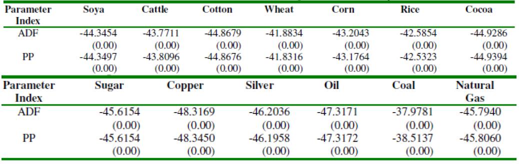
Finally, the application of standard modelling techniques and conventional diagnostics as mentioned in Alexander (2001) is endorsed by the Augmented Dickey-Fuller (ADF) and Philips-Perron (PP) reported in Chart 7. Both values comfortably exceed the critical values at 1%, 5% and 10%, signifying that the unit root null is categorically rejected in favour of stationary mean-reverting return series in all the examples analysed.
6. Basel II framework. Panorama before and up to the Subprime Crisis
6.1.1. Backtesting and Performance of VaR Models
Charts 8 and 9 exhibit the outcome of the Backtesting for the VaR models enunciated in Section 4.3 recorded in 2008. As it should be expected, HS underestimates the risk and reports disappointing results translated in seven Red Zones, four Yellow and -quite surprisingly-a Green one (natural gas). However, both the Yellow and the Green Zones do not dissipate the gloom on the technique as the quantity of exceptions situates on the brink of the Red Zone (9 for soya and 8 for rice, copper and silver), whereas the latter constitutes the only series to report Green zones for all the specifications
Chart 8: Backtesting -Quantity and proportion of exceptions in forecast period
Note: Student-t models are excluded as they hit convergence problems for coal (the degrees of freedom equalled 2).
Chart 9: Backtesting The Three Zone Approach - Increase in scaling factor k
Note: Student-t models are excluded as they hit convergence problems for coal (the degrees of freedom = 2)
The application of the conditional volatility filters (GARCH and EGARCH) brings about a change in the panorama with relevant aspects to analyse. Setting aside all the specifications featuring the Student-t for coal (Section 5.2), it leaps to the eye that the outcome matches more closely the heteroscedas- tic nature of the time series, although a closer look reveals that a somewhat disappointing pattern for the EGARCH model, for both FHS and CV variants. In effect, the FHS/GARCH-N records four Green Zones (soya, rice, silver and natural gas), with one red (sugar) and the remaining ones Yellow, whereas the FHS/GARCH-t only adds copper to the non-penalty category despite the heavier tails embodied in the Student-t distribution. On the other hand, FHS-EGARCHs behave less accurately than its counterparts. In effect, FHS/EGARCH-N posts only three Green Zones (soya, rice and natural gas) with four Red (cattle, wheat, corn and coal) and five Yellow. FHS/EGARCH- t records slightly better outcomes: four Green Zones (soya, rice, copper and natural gas), two Reds (wheat and corn), five Yellows and one invalid (coal). The situation appears faintly reversed on the CV camp as the performance of the Normal models (GARCH and EGARCH) deteriorates while the Student-t bound ones recovers. CV/GARCH-N offers only two Green Zones (rice and natural gas), two Reds (cocoa and sugar) and the remaining eight Yellows while the Student-t variant behaves astonishingly well featuring seven Greens, five Yellows and one invalid. On the other hand, CV/EGARCH-N places itself even behind HS in terms of Red Zones (eight), delivering only three unpenalised series (soya, rice and natural gas), and two commodities to be scrutinised. CV/EGARCH-t brings about a satisfactory result: six Greens, one red (wheat), five Yellows and one invalid (coal). On the grounds of the aforementioned results, CV/GARCH- t seems to situate an inch ahead of the rest FHS/GARCH-t in terms of the overall performance, although the gap is far from conclusive. Notwithstanding that, there may be evidence of the fact that the model (GARCH) influences the performance when the filtered empirical distribution is employed to calculate the quantile (i.e., VaR), whereas the distribution is more relevant at the time of affixing a theoretical density (Student-t) to the detriment of the representation.
Finally, reveals as the most reliable scheme, as it delivers thirteen Green Zones, obviously as a product of higher VaRs, again enhancing its reputation as the most consistent technique capable of dealing with market crises.
6.1.2. Backtesting and Capital Levels
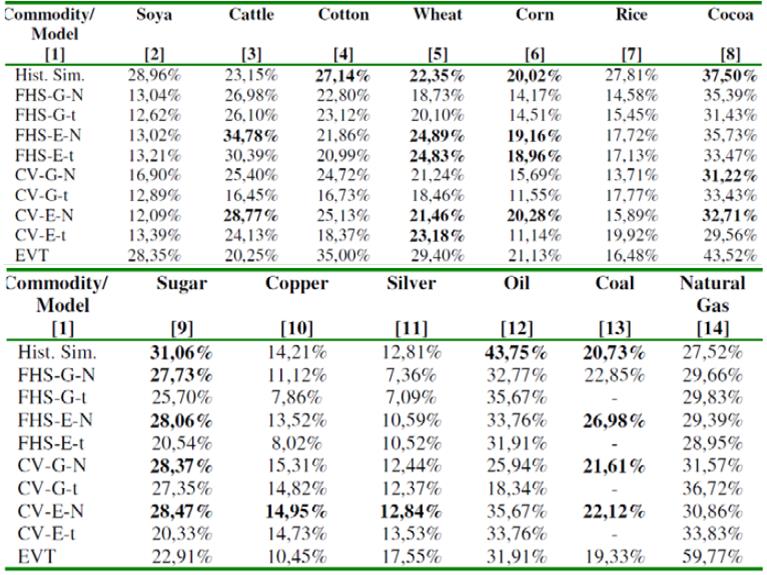
As displayed in Chart 3, the outcome of Backtesting plays a central role in the determination of the MCR, accompanied by the 60-day average VaR rule (formula 3.1). From Chart 9, the absence of surcharges in Backtesting rewards EVT as the most trustworthy scheme, whereas, on the other hand, HS and CV/EGARCH-N, featuring seven and eight Red Zones respectively, champion the less reliable ones 19 (Columns 1 and 10). However, the rest of the models deliver mixed performances which blur any neatly drawn distinction among them, though under relatively high add-on factors over the 40% floor. 20
Intra-series comparison understandably shows that the application of the leptokurtic Student-t distribution improves the results diminishing the penalties both for GARCH and EGARCH specifications in FHS and CV environments 21 (Columns 2 vs 3, 4 vs 5, 6 vs and 8 vs 9) In general terms it is noteworthy to reinforce one of the assertions in Section 6.1.1 regarding the prevalence of the models over the shape of the distribution in FHS and viceversa in CV: FHS/GARCH-N equations beat FHS/EGARCH-N ones for cattle, wheat, corn, copper, oil and coal (40% ≤ k ≤ 85% against 50% ≤ k ≤ 100% in Columns 2 and 4) whilst the both specifications dispute the contest under the Student- t distribution (FHS/GARCH-t comes out first for cattle, corn, silver whereas its counterpart does the same for cotton, wheat, sugar and oil, albeit in both occasions bearing elevated penalties. On the contrary, usage of the Student-t distribution brings about a dramatic improvement wrt the Gaussian assumption under the CV regime: Columns 6-7 and 8-9 exhibit that CV/GARCH-t and CV/EGARCH-t obtain seven and six Green Zones respectively against two and three of CV/GARCH-N and CV/EGARCH/N respectively. CV/GARCH- t gets only one considerable extra charge (75% for cocoa) while CV/GARCH-N delivers three k=85% (cattle, wheat and copper) and two 75% (cotton and silver). The outlook appears more compromised for CV/EGARCH-N because of its eight Red Zones vs one of CV/EGARCH-t (wheat).
MCR exhibited in Chart 10 denote a relatively levelled panorama with few scattered outliers in EVT in terms of the quantity demanded (there is a difference of 101% for soya, 77% for cotton, 71% for corn and 74% for silver between EVT's MCR and the second higher MCR belonging to the Green Zone). It is less clear that models belonging to the Green Zone should build higher MCR than those subject to penalties because, after allowing for EVT for soya, cotton, wheat, corn, cocoa and silver, the remaining unpunished e.t. techniques (and, in some occasions, EVT) manage to constitute capital cushions lower than or almost levelled with those of the smallest Yellow Zone MCR (irrespective of the specification rendering it): CV/GARCH-t and EVT for cattle, CV/GARCH-t and CV/EGARCH-t for cotton and corn, all FHS, CV and EVT for rice, EVT for sugar, FHS/Gt, FHS/E-t and EVT for copper, FHS/G-N and FHS/G-t for silver and CV/GARCH-t. CV/EGARCH-t and EVT for oil. There are only few cases when schemes well into the Yellow Zone end up constituting less MCR than the ones belonging to the Green Zone: 22 FHS/GARCH-N (50%, 29.80%), FHS/GARCH-t (65%, 33.78%), CV/GARCH- N (85%, 34.44%), CV/GARCH-t (50%, 30.36%)vs EVT (0%, 47.67%) for wheat (Chart 10, Column 5) and FHS/GARCH-N (85%, 39.30%), FHS/GARCH- t (65%, 36.23%), FHS/EGARCH-N (75%, 33.48%), FHS/EGARCH-t (65%, 32.94%), CV/GARCH-t (75%, 35.70%) and CV/EGARCH-t (50%, 29.29%) against EVT (0%, 46.34 %).
Chart 10: Minimum Capital Requirements VaR MCR(VaR) - M CR 2 Basel II directives
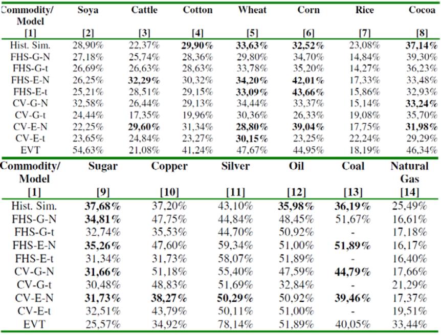
Notes: (1): Values in bold letters indicate specifications belonging to the Red Zone to be eventually excluded by regulators. (2): Student-t models are excluded as they hit convergence problems for coal (the degrees of freedom = 2).
6.1.3. The Simplified Approach and Capital Requirements in Basel II
Although the existence of SA may be partly justified, 23 it use for MCR calculation purposes has been a contentious issue since its inception (Penza and Bansal (2001) and Prescott (1997)). 24 In effect, under Prescott's framework (1997) 24 an entity enters bankruptcy when market losses exceed capital provisions; therefore, healthy institutions would endeavour to keep their excessions record at 0. However, the 18% flat rate (as opposed to the mandatory 8% for equity) constitutes a more adequate threshold as the appreciation of Chart 11 conveys. In effect, had the SA been adopted, only positions in soya would have driven banks to bankruptcy (one exception); therefore, the application of the current scheme (which basic rate is increased in 87.50% compared with stocks) warrantees, in principle, banks' financial health in risky scenarios and vindicates its inclusion in Basel II.

6.1.4. Basel II, Moral Hazard and Incentives
Sections 6.1.1 to 6.1.3 aimed at describing the behaviour of the different IM VaR-based models and the SA and the respective derived MCR during market turmoil. In this sense, according to the sample and forecast periods selected, the presence of moral hazard does not appear crystal clear as there are not many instances when models well into the Yellow Zone yield higher MCR than those in the Green Zone (Chart 10).
In effect, setting aside EVT for soya, corn and silver when the amounts of MCR could be labelled as outliers, series belonging to wheat and cocoa deliver traces of moral hazard given that -excluding disallowed techniques- FHS/GARCH-N (k=50%), FHS/GARCH-t (k=65%), CV/GARCH- N (k=85%) and CV/GARCH-t (k=50%) for the former and FHS/GARCH-N (k=85%), FHS/GARCH-t (k=65%), FHS/EGARCH-N (k=75%), FHS/EGARCH-t (k=65%), CV/GARCH-t (k=75%) and CV/EGARCH- t (k=50%) for the latter render lower MCR compared to the unpunished EVT. For the rest of the commodity series, it is possible to find a Green model able to dodge the moral hazard trap: soya (FHS/GARCH-N, FHS/GARCH- t, FHS/EGARCH-N, FHS/EGARCH-t, CV/GARCH-t, CV/EGARCH-N and CV/EGARCH-t), cattle (CV/GARCH-t and EVT), cotton (CV/GARCH-t and CV/EGARCH-t), corn (CV/GARCH-t and CV/EGARCH-t), rice (all representations but HS), sugar (EVT), copper (FHS/GARCH-t, FHS/EGARCH-t and EVT), silver 25 (FHS/GARCH-N and FHS/GARCH-t), oil (CV/GARCH-t) and coal (EVT).
The adoption of the SA does not entirely play to the detriment of the IM approach considering that it does not always deliver the lowest MCR, undoubtedly due to the 87.50% increase in the former. In this vein, Charts 12 and 13 , which feature the average MCR for the year 2008 and the relative difference over the SA (fixed at 18%) during that period, eloquently display that, on average terms, 26 the SA does not always yield the lowest MCR. Surprisingly enough, the alternate positive and negative signs in Chart 13 evince that for specifications lying in the Green or Yellow Zones it is possible that the capital cushion should be lower than SA 27 the figures exhibited in Chart 12 and 13 do not, then, appear to convey a significant underestimation of risk.
Chart 12: Average MCR 2 for Year 2008 VaR MCR(VaR) - Basel II Directives

Notes: (1):Values in bold letters indicate specifications belonging to the Red Zone to be eventually excluded by regulators. (2):Student-t models are excluded as they hit convergence problems for coal (the degrees of freedom = 2).
Chart 13: Average MCR 2 for Year 2008 VaR MCR(VaR) - Increase over SA - Basel II directives
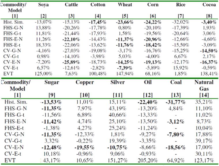
Notes: (1):Values in bold letters indicate specifications belonging to the Red Zone to be eventually excluded by regulators. (2):Student-t models are excluded as they hit convergence problems for coal (the degrees of freedom = 2).
Consequently, even though traces of moral hazard still hover in the background, the evidence gathered emphatically denies the lack of incentives to develop accurate models to build enough capital requirements to fend off market crises of considerable magnitudes.
7. Basel III: The Regulatory Response to The Crisis
7.1. The impact of the Introduction of the sVaR
The capital charges brought about by Chart 14 as a result of the sVaR exercise bear a great deal of resemblance to Basel II's outcome (Chart 11). EVT again generates the highest MCR for cotton, wheat, corn, cocoa, silver and natural gas irrespective of the Backtesting allocation of the rest of the specifications which erects moral hazard as a major deterrent to develop accurate schemes. EVT's plight turns particularly worrisome for cotton, corn and silver as the remaining Green models manage to escape unscathed.
Chart 14: Basel III Minimum Capital Requirements Internal Model Approach (sVaR)
Notes:(1):Values in bold letters indicate specifications belonging to the Red Zone to be eventually excluded by regulators. (2):Student-t models are excluded as they hit convergence problems for coal (the degrees of freedom = 2).
Chart 15 reports Basel III's total capital charge as a result of the sum of the components stated in (3.2), from where it could be appreciated that the BCBS finally achieves its declared aim of strengthening the capital base, providing banks a substantial war chest to avert huge market turbulence. Three immediate observations arise from Chart 15 and Chart 16 -informative of the rise in percentage with reference to Basel II MCR-: in the first place, the increases appear to situate on similar relative values (except coal); secondly, the relative variations as a result of the application of sVaR appear truly huge and, finally, the level of minimum capital required seem somewhat colossal.
Like for Basel II, Basel III still presents traces of moral hazard. In effect, Chart 15 hints at its appearance for wheat, where FHS/GARCH-N, FHS/GARCH-t, CV/GARCH-N and CV/GARCH-t manage to deliver lower MCR than EVT despite bearing surcharges of 50%, 65%, 85% and 50% respectively and cocoa, with FHS/GARCH-N (85%), FHS/GARCH-t (65%), FHS/EGARCH-N (75%), FHS/EGARCH-t (65%), CV/GARCH-t (75%) and CV/EGARCH-t (50%) rendering lower values than the unpunished EVT. Un- fortunately, despite the outstanding behaviour showed in Backtesting, EVT's based MCR augments 62% and 94% for wheat and cocoa, with the remaining specifications rising in similar proportions. The overall panorama remains mostly unchanged for the remaining eleven commodities, including two distinctive features: the existence of a Green technique yielding less capital than the first Yellow one, thus implying absence of moral hazard and finally, the huge increase in equity levels disregarding the Backtesting Zone.
Chart 15: Minimum Capital Requirements VaR MCR(VaR) - MCR 3 Basel III directives
Notes:(1):Values in bold letters indicate specifications belonging to the Red Zone to be eventually excluded by regulators. (2):Student-t models are excluded as they hit convergence problems for coal (the degrees of freedom = 2).
Chart 16: Increase in MCR = MCR 3 / MCR 2
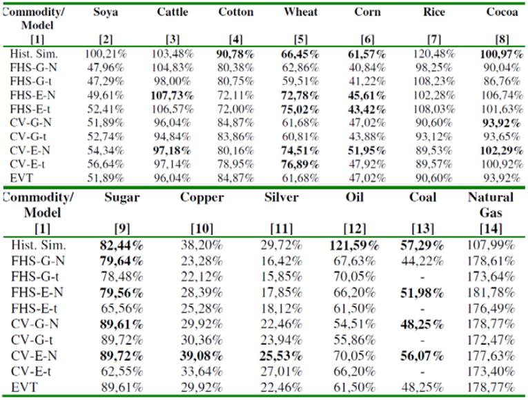
Notes:(1):Values in bold letters indicate specifications belonging to the Red Zone to be eventually excluded by regulators. (2):Student-t models are excluded as they hit convergence problems for coal (the degrees of freedom = 2).
MCR augments 62% and 94% for wheat and cocoa, with the remaining specifications rising in similar proportions. The overall panorama remains mostly unchanged for the remaining eleven commodities, including two distinctive features: the existence of a Green technique yielding less capital than the first Yellow one, thus implying absence of moral hazard and finally, the huge increase in equity levels disregarding the Backtesting Zone. Although EVT has been specially designed to respond to unforeseen abrupt market turmoil -consequently delivering Green Zones for every commodity series, the application of Basel III mandates may end up storing unnecessarily elevated capital cushions leading to unproductive inefficient uses. However, banks should deal with the enticement to apply less accurate models with the utmost care in view of the inconsistent Backtesting outcome.
7.2 The SA and Basel III:old sins have long shadows
Sections 3.2.1 and 3.3.2 pointed out that Basel III cracked down on IM leaving SA invariant. As it could be surmised, it plays to the detriment of any VaR model, assertion confirmed by Chart 17 which pictures the percentage increase in MCR after the application of the sVaR wrt the SA. Banks selecting IMA would be compelled to set aside staggering additional buffers 28 between 99% (rice) and 342% (oil), hence giving birth to a host of disincentives to adopt the IM under Basel III framework.
8. Basel Capital Accords and the (dis)incentives to develop IM
Sections 6.1.1, 6.1.2, 6.1.4 and 7.1 signalled the prowess of EVT to deal with unforeseen adverse market events in both Basel II and Basel III configurations. However, that security comes at the expense of somewhat high VaR values which, in turn, reflect in relatively elevated MCR, sometimes well above the second model in the Green Zone pecking order. On the grounds of the bright performance of EVT, 29 this Chapter inquires about the motivation to employ precise VaR techniques, hinting at potential alternatives to implement Basel III keeping the accuracy incentives aligned between the IM and SA appraisals. The sensitivity analysis suggests that Basel III might have been applied somewhat differently.
8.1. Basel II and the Role of the Multiplier Factor mc Revisited
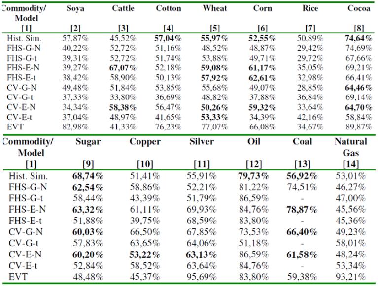
Some interesting observations seem to be conveyed by Charts 18 and 19. EVT-derived MCR2 would have shielded banks against daily losses spanning 1.60 (rice) to 5.64 (wheat) times the maximum loss of the backtesting year 2008 (translating into 18% and 48% shortfalls respectively) as displayed in Chart 18, Column 2 under the heading Loss Coverage (LC) 30 In terms of the highest daily losses, Chart 18 Column 3 informs that positions in silver and soya could afford to plummet 78.14% and 54.63% (Loss Coverage of 5.61 and 2.33). These equity cushions constitute the logical defence to periods of high volatility (Brooks, Clare and Persand (2000)), as Chart 19 -Columns 2 to 4-implies, given that all series but natural gas recorded either moderate or huge hikes in their variability, from 14% (cattle) to 153% (coal), meaning daily losses in the interval 8% (corn) to 23% (soya).However, Columns 4and 5 in Chart 18 exhibit that EVT would still have shielded banks against the highest loss in the sample period (18.19%, LC=0.74 for rice and 82.71%, LC=5.61 for silver).
Chart 18:.Basel II MCR2-Loss coverage and Maximum daily loss
Note: Loss coverage = MCR2 / Maximum loss forecast period Loss coverage(*) = M CR 2 / Maximum loss sample period
Danielsson, Hartmann and de Vries (1998) identified the size of the multiplication factor mc as one of the chief snags of Basel II, and although it being set at 3 may help to provide financial institutions enough MCR to fend off Taleb's 'black swans' (2007), it can also leave the door of moral hazard ajar. In this sense, Chart 20 portrays a sensitivity analysis that compares values of MCR (tantamount to the maximum daily losses allowed) alongside the maximum Loss coverage for alternative values of mc employing the highly leptokurtic EVT. The outcome, then, eloquently indicates that mc=3 is susceptible to yield excessive MCR given that, for instance, a 23% reduction in mc (mc=2.30) would yield an average 35% MCR enough to raise the Loss Coverage to more than 3 (Chart 20, Columns 2 and 3). Furthermore, a more aggressive cut to mc (i.e., 33%), which reduces mc to 2 could also take place, as it would render average MCR of 30.41%, equivalent to an average LC=2.62 (Chart 20, Columns 42 and 43).
Chart 20: Sensitivity Analysis - MCR 2 and Loss coverage with varying factor mc - EVT-derived values

Note: Loss coverage = MCR 2 / Maximum loss forecast period
In view of the aforementioned evidence, Basel II does not seem to foster the application of the IM appraisal. Chart 11, Column 4, indicates that theLC obtained from the application of the SA reaches, on average terms, 1.76 31 (MCR=18% -flat rate-). While under very unusual market circumstances, SA could not grant survival, the scenario does not look so dramatic, courtesy of the 87.50% increase in the fixed proportion. There is, then, a sense of disadvantage to IM, particularly the most accurate ones, although the moral hazard arising from that fact appears somewhat circumscribed on the grounds of the rather satisfactory performance of the SA. Mechanisms that ameliorate the extent of the moral hazard would require a drastic reduction of the mc multiple of more than 33%, possibly to some level between the interval [1,20; 1,35] where the MCR would average between 18% and 21%, and the respective LC situate in the bracket [1,57; 1,77], in line with the SA 32 (Chart 20, Columns 68 to 75).
8.2. Basel III and the Role of the Multiplier Factors m c and m s revisited
As Section 7.1 implied, the enactment of the stressed term undoubtedly attained the purpose intended: Columns 2 and 4 in Chart 21 evince that the LC grows, on average terms, 60%, from 3.91 to 6.27 (3.05 and 10.38, minimum and maximum losses for rice and natural gas respectively), eventually representing daily losses of 35% (cocoa) and 96 % (silver).
Chart 21: Basel III MCR 3 -Loss coverage and Maximum daily loss Variation over MCR 2
Note: Loss coverage = M CR3 / Maximum loss forecast period
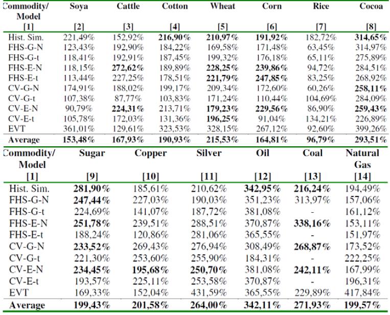
On the grounds of the results obtained for Basel III configuration, Chart 22 informs the outcome of the sensitivity analysis -expressed in terms of the MCR or, equivalently, the maximum daily loss-employing different combinations of the factors m c and m s . It leaps to the eye that the adoption of Basel III would unnecessarily immobilise huge amounts of capital, thus raising inefficiency concerns as they could be allocated to more productive uses (Chart 22, line 30). Therefore, one likely alternative to mitigate the degree of that distortion while conserving the current structure boils down, again, to downgrade the size of the multipliers mc and ms with a view to finding a more satisfactory combination.
Chart 22: Sensitivity Analysis -Total MCR with varying factors mc and ms -EVT-derived values
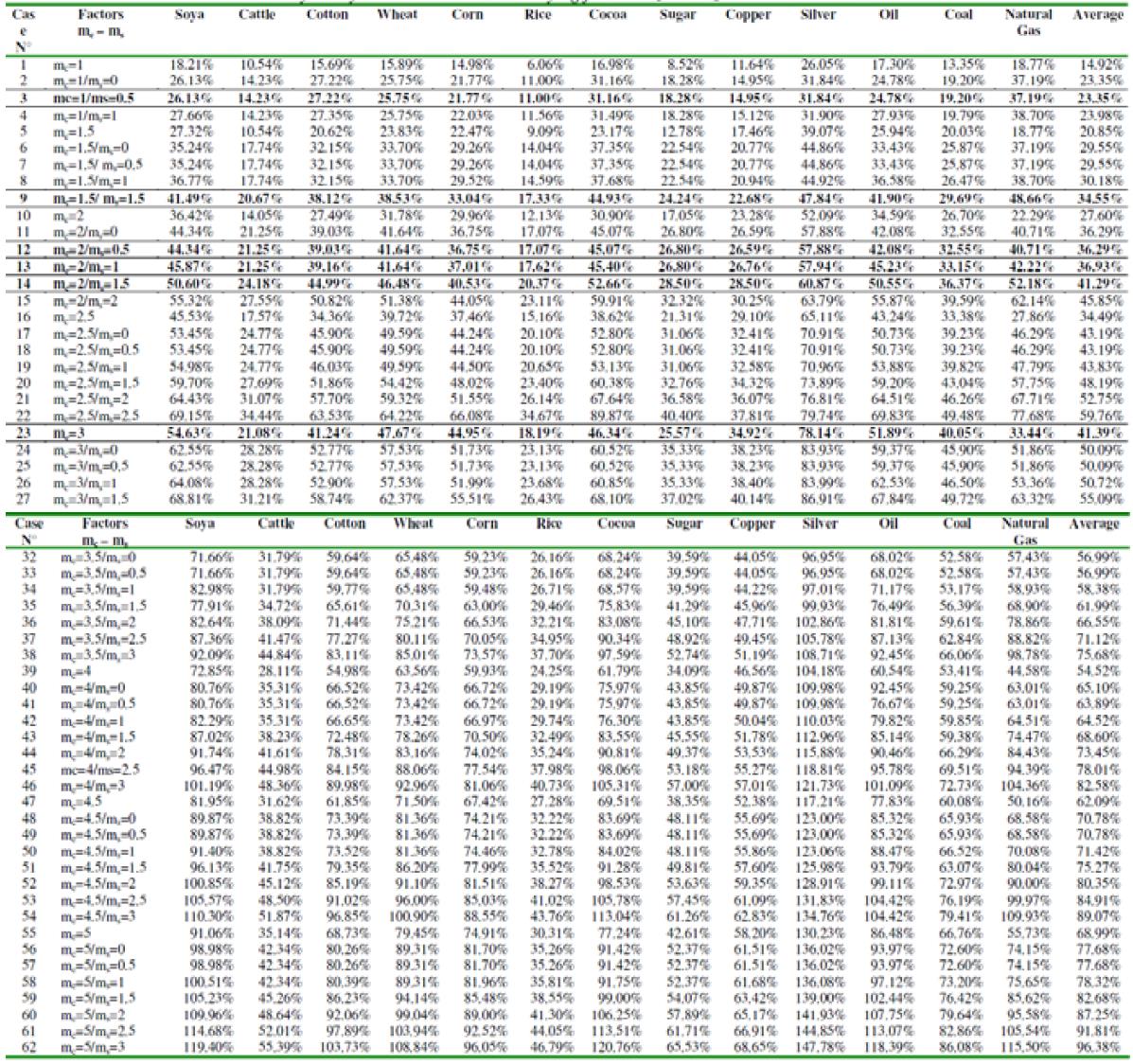
Notes: (1): Cases 3, 9, 12, 13 and 14 highlighted in bold letters as referenced in main text. (2): Cases 23 and 30 correspond to Basel II and Basel III directives respectively.
Even though the decision appears not devoid of any subjectivity in the final assessment, it may be the case that mc should not be greater than 2, whereas its counterpart m s could take some values in the interval [0,5; 1,5] (Chart 22, lines 12 to 14), hence M CR ∈ [36%; 41% ], tantamount to an average LC between 3.49 and 3.98 (Chart 23, Columns 6 to 11) which represent variations from the Basel II's MCR in the bracket [-9%; +3% ] (Chart 24, Columns 6, 8 and 10) and, in terms of Basel III, a decrease between 37% and 43%, still providing adequate coverage for abnormal market movements (Chart 24, Columns 7, 9 and 11).
There may exist, however, other viable alternatives like m c = 1.5 and m s = 1.5 which could drive the average MCR to 34% and the corresponding average LC to 3.35 (decreasing MCR2 and MCR3 in 13% and 50% respectively) (Charts 23 Columns 4 and 5, and Chart 24 Columns 4 and 5). Finally, many complications surge at the time of finding the equivalence between the EVT-based IM and the SA: the pair m c = 1, m s = 0.5 might, allowing for some flexibility, bring the MCR near the 18% flat rate characteristic of the latter, though still above (particularly for cocoa, silver and natural gas as conveyed by Chart 22, line 9). Consequently, it remains to be seen which incentives banks may find to employ accurate models like EVT when the easiest route to MCR constitutions do constitute a reasonable fence against violent market turmoil.
Chart 23: Sensitivity Analysis - Selected examples. Loss coverage and Maximum Daily Loss

Note:(1): Loss coverage [2],[4], [6], [8], [10] = MCR 3 / Maximum loss forecast period.
9. Final remarks
In general terms, after the collapse that many financial institutions experienced as a consequence of the subprime crisis of 2008, the reinforcement of the capital base seems an unquestionably wise strategy. The proofs collected mark that, after the introduction of the sVaR, the CCB and CyCB, the BCBS would attain the objective.
The current study underlines some policy implications that may result in Basel III having included some different provisions regarding the MCR for the trading book. Even though the evidence might allow some sort of condescension with techniques featuring the Normal or even some Student-t distributions, their inconsistent performance could render them unreliable for MCR determination purposes. In that vein, the numerical exercise again shows that EVT retains the leadership at the time of shielding banks against abrupt adverse market swings, although generalisations regarding a likely pecking order remain wide off the mark. It is deemed, then, that the BCBS should disallow permanent underperforming schemes like HS and recommend the employment of (highly) leptokurtic models which excel in Backtesting, ideally EVT or, under careful scrutiny, some Student-t ones with low degrees of freedom.
Danielsson, Hartmann and de Vries (1998) pointed out that one of the major flaws of Basel II, connected with the treatment of market risks, stemmed from the value of the multiplication factor m c . The present article delves into the matter only to uphold the previous inferences for commodity portfolios, given that m c = 3 imposes an arguably excessive capital levy, which, in the event of utilising leptokurtic models like EVT, derives in an unnecessary immobilisation of resources. The sensitivity analysis exhibited that mc below 2 would have shielded banks against market blows of huge magnitudes, thus implying a reduction in the value of mc of approximately 33% and still providing sizeable coverage.
Additional repercussions are brought about by the application of the stressed component in the MCR formula corresponding to Basel III. Considering the aforementioned conclusions about Basel II, the mandate to use ms renders the MCR disproportionate for models complying with Backtesting to the letter, i.e., falling under the Green Zone. Acknowledging the fact that Basel III is currently being in implementation, the article ventures to suggest the dissociation of the values of the factors mc and ms and the possibility to assign them alternative values in accordance to the prowess of the scheme used could constitute a likely attempt to ease the burden on accurate models and, simultaneously, encourage banks to develop them. The current paper hints at several combinations between mc and ms which would save banks from large scale plights, eventually at the discretion of national or supranational regulators after more comprehensive studies with different samples; however, setting m c = 1.5 and m s = 1.5 or, giving financial institutions some sort of leeway in ascertaining the proper value of mc in the interval [1.5; 2] with ms belonging to [0.5; 1.5] convey an idea about the kind of approaches that may keep incentives for accuracy.
The right motivations for accuracy immediately direct the attention to the existence of the SA (or, to some extent, the MLA). The dual criterion triggers the incentives issue much like in Rossignolo, Fethi and Shaban (2012), albeit in a somewhat different fashion as the situation verified for commodity markets could be regarded as healthier through the prism of the right incentives to adopt sound approaches. The evidence garnered exhibited that VaR models almost always deliver MCR higher than those given by the SA but only once was a capital shortage verified. Therefore, even though banks may feel inclined towards SA, the 18% demanded for commodities (representing an extra 87.50% in comparison with stocks) does not automatically lead to bankruptcy, hence mitigating the upsurge in moral hazard and making this recipe appealing for other kinds of exposures like equity.
The fact that the application of sharp leptokurtic models like EVT would have vindicated Basel II framework and, furthermore, that different values of m c (Basel II) and different combinations of m c and m s would have yielded Basel III less punitive on responsible banks brings about interesting policy implications. Applauding the decision to increase the capital levels, and, in this sense, agreeing that the hike in SA reduces the risk of ruin after its adoption, it is believed that the whole configuration is still a bit unfair on IM. The article puts forward a feasible and relatively easy solution characterised by the modification of the values of the parameters mc and ms subject to the employment of a leptokurtic model, ideally EVT, in order to: a) provide enough protection against market turmoil and b) keep accuracy incentives aligned with SA. In this sense, were banks allowed to reverse to Basel II framework, m c could be assigned some value between [1.20; 1.35] whereas if Basel III reached an irreversible stage, m c and m s may take figures near 1 and 0.5 respectively. Granting national regulators with some margin to equate the appraisals - conditional on the usage of restricted models-is judged as a step in the right direction to reduce the moral hazard while simultaneously safeguarding a capital buffer sufficient to secure the survival in troubled markets.

