


Services on Demand
Journal
Article
 English (pdf)
 Article in xml format
 Article references
 Send this article by e-mail
Indicators
-
 Cited by SciELO
 -
 Access statistics
Related links
-
 Similars in
SciELO
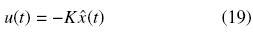
Similars in
SciELO
Share

 Permalink
Revista mexicana de ingeniería química
Print version ISSN 1665-2738
Rev. Mex. Ing. Quím vol.10 n.3 Ciudad de México Dec. 2011
Simulación y control
Control of second order strictly proper unstable systems with time delay
Control de sistemas inestables estrictamente propios de segundo orden con retardo
D.F. Novella–Rodríguez and B. del Muro–Cuéllar*
Escuela Superior de Ingeniería Mecánica y Eléctrica, Unidad Culhuacan, Instituto Politécnico Nacional, México, D.F., 04430, México. *Autor para la correspondencia. E–mail: dnovellar@gmail.com
Received 17 of March 2011.
Accepted 25 of September 2011.
Abstract
This paper considers the stabilization and control of linear time invariant systems containing two unstable poles, a "stable" zero and time delay. It is well known that time delays complicate the stability analysis and the design of appropriate control strategies. For this reason, we propose a simple control strategy based on an observer system with the aim of stabilize this class of systems. Necessary and sufficient conditions are stated in order to guarantee trie stability of the closed loop system. Once the stability conditions are satisfied, only the plant model and four proportional gain s are enough in order to implement the proposed control strategy. Finally, some examples are presented in order to illustrate the proposed control strategy performance, showing some robustness when uncertainties are presented in thetime delay value.
Keywords: time–delay, unstable systems, stabilization, observer, linear systems.
Resumen
El presente trabajo considera el problema de la estabilización y control de sistemas lineales e invariantes en el tiempo que contienen dos polos inestables, un cero "estable" y tiempo de retardo. Es conocido que los retardos complican el análisis de estabilidad de los sistemas así como el diseño de estrategias de control adecuadas. Por esta razón, se propone una sencilla estrategia de control basada en un sistema observador con la finalidad de estabilizar esta clase de sistemas. Se presentan condiciones necesarias y suficientes que garantizan la estabilidad del sistema en lazo cerrado. Una vez satisfechas dichas condiciones, sólo el modelo de la planta y cuatro ganancias proporcionales son necesarias para implementar la estrategia de control propuesta. Finalmente, se presentan algunos ejemplos con la finalidad de ilustrar el desempeño de la estrategia de control propuesta, mostrando cierta robustez cuando se presenta incertidumbre en la dimensión del tiempo de retardo.
Palabras clave: retardo, sistemas inestables, estabilización, observador, sistemas lineales.
1 Introduction
Time–delay is the property of a physical system by which the reponse to an applied signal is delayed in its effect. Systems with delays are very common in the world, they appear in various systems as biological, ecological, social, engineering systems, etc. and are due to several mechanisms like material or energy transport, recycling loops, etc. In addition, actuators, sensors and field networks that are involved in feedback loops usually introduce such delays, (Zhong, 2006)). Also delays can be used in modeling reduction where high–order (finite–dimensional) systems are approximated (in some norm sense) by low order systems with delays, (Skogestad, 2003).
It is well known that time–delay is often a source of complex behaviors (oscillations, instability and bad performance) in many dynamic systems. Thus, considerable attention has been paid on this kind of systems in order to understand how the delay term may deteriorate the behavior of the system and to control their effects for achieve a better performance on closed–loop systems, (Niculescu, 2001, Gu et al. 2003, Richard, 2003).
Several control strategies have been developed to deal with delayed systems. A common approach is to approximate the time–delay operator by means of a Taylor or Padé series which could leads to a non–minimum phase system with rational transfer function representation. Another classical control approaches for time–delay systems includes Proportional Integral Derivative (PID) control, classical smith predictors (SPC), etc., (Smith, 1957, Palmor, 1996, Silva et al., 2004).
Open–loop unstable processes arise frequently in chemical and biological systems and are fundamentally difficult to control. Unstable time–delay systems represent a challenge for control design, for instance, the SPC scheme does not have a stabilization step, which restricts its application to open–loop stable plants. To get over this problem, some modifications of the SPC original structure have been proposed to deal with non–stable delayed process, for instance, Rao et al. (2007) have presented an efficient modification to the Smith predictor in order to control unstable first order system plus time delay. With a different perspective, Normey–Rico and Camacho (2008) propose a modification to the original Smith structure in order to deal with unstable first order delayed systems. Using a similar structure, the result is extended to delayed high order systems in Normey–Rico and Camacho (2009). In both papers, a robustness analysis is done concluding that for unstable dead time dominant systems, the closed–loop system can be unstabilized with an infinitesimal value of modeling error, i.e., that robustness is strongly dependent on the relationship τ/τun, where τ is the process time delay and τun is the dominant unstable time–constant. For the control scheme proposed in these later two papers, it can be easily proven that in the case of unstable plants, the internal stability is not guaranteed. In fact, an unstable estimation error is obtained and, as a result, even a minimal non zero initial condition at the original plant or in the controller, produces an internal unbounded signal. Notice that in a practical situation it is not possible to exactly measure the initial condition of the plant to assign the same value to the model considered on the modified Smith compensator.
Following the same idea of the Smith predictor, in del–Muro–Cuellar et al. (2007) it is proposed an observer based controller, but designed by mean of a partition and a Padé approximation of the delay term. It is important to note that the results in that paper seems to be adequate for the numerical examples presented, but there are no formal results considering the maximal size of delay that can be accepted. In this way, in Marquez et al. (2010) an observer based control structure is proposed and necessary and sufficient conditions in terms of the delay length are stated for the stabilization and control (step tracking and disturbance rejection) of delayed systems. However, this result is restricted to first order systems.
Nevertheless, many chemical and biological systems present second–order behavior. Continuous stirred tank reactors, polymerization reactors and bioreactors are inherently unstable by design; this type of systems can be modeled as open–loop unstable second order plus time delay models, (Rao and Chidambaram, 2006, Shamsuzzoha et al., 2007).
In this work it is proposed a simple control strategy based on an observer based schema with the aim of stabilize unstable second–order systems with delay at the input – output direct path. In particular, plants including one "unstable" zero are considered. Necessary and sufficient conditions in order to guarantee the stability of the closed loop system are stated. The stabilizer structure relies on an observer–based structure with a memory observer and a memory less state feedback. On the contrary of modified Smith predictors, the scheme only contains discrete time delay (and not distributed ones) which makes easy its practical implementation (see Zhong, 2006, for details on numerical implementation of modified Smith predictor scheme).
This paper is organized as follows; Section 2 is dedicated to the problem formulation. The Section 3 yields the preliminaries results used to obtain the main result of this work. An observer based controller is proposed in Section 4, in order to stabilize the unstable second order systems without zeros. In the main Section 5, necessary and sufficient stability conditions for the proposed controller scheme are stated for systems including one "stable" zero. Then, in Section 6 numerical simulations are presented in order to illustrate the controller performance. Finally some concluding remarks are stated in Section 7.
2 Problem statement
Consider the following class of single–input single–output (SISO) linear systems with delay at the direct path:
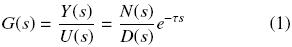
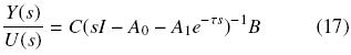
where U (s) and Y (s) are the input and output signals respectively, τ > 0 is the time delay, N(s) and D(s) are polynomials in the complex variable s and G(s) is the delay–free transfer function. Notice that with respect to the class of systems (1) a traditional control strategy based on an output feedback of the form

produces a closed–loop system given by:
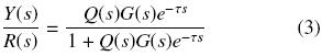
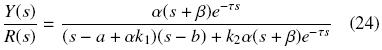
where the exponential term e–τs located at the denominator of the transfer function (3) leads to a system with and infinite number of poles and where the closed–loop stability properties cannot easily be stated. From the classical structure of the Smith predictor (SPC) given in Fig. 1, it is known that the transfer function of the closed–loop system is obtained as follows:
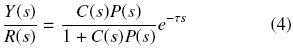
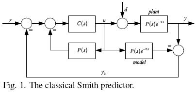
It can be noticed that the delay term is shifted outside of the characteristic equation of the system. Under ideal conditions, i.e., exact knowledge of the plant parameters, the SPC provides a successful future estimation time units ahead of the y(t) signal, which could be used like a control signal in a specific feedback scheme, (Smith, 1957, Palmor, 1996). Unfortunately, the classical structure of the SPC is restricted to stable processes. Different authors have proposed several modifications to the original SPC structure to give solution to some particular cases, (Normey–Rico and Camacho, 2008, Normey–Rico and Camacho, 2009, Rao et al., 2007, Zhong, 2006).
As was mentioned above, a minimal initial condition difference between the original plant and the model produces an internal unbounded signal, which can be produce instability in practical situations.
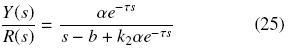
This work proposes an observer based control scheme in order to stabilize an unstable second order system characterized by the following transfer function:
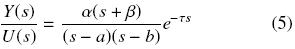
where, without loss of generality, a > b > 0 and β,τ > 0.
3 Preliminary results
Preliminary results are presented here. They will be used later in order to state the stability conditions of the studied system. Let us consider the following unstable first order system plus time delay
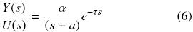
with a > 0; and a proportional output feedback control as follows:

This produces the closed–loop system:
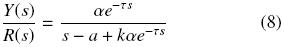
The following result has been widely studied in the literature and the proof can be easily obtained by considering different approaches as a classical frequency domain. An alternative simple proof based on a discrete time approach is shown in Márquez et al. (2010).
Lemma 1. Consider the delayed system (6) and the proportional output feedback (7). Then, there exists a proportional gain k such that the closed loop system (8) is stable if and only if τ < a–1.
Now, consider the system characterized by:
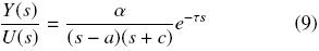
with a, c > 0. Note that the system has only one "unstable" pole. With the proportional output feedback given by Eq. (7), we get a closed–loop system as follows:
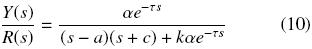
Lemma 2. Consider the delayed system (9) and the proportional output feedback (7). Then, there exists a proportional gain k such that the closed loop system (10) is stable if and only if τ < a–1 – c–1.
The proof of this result can easily be obtained by mean of different approaches, as the frequency domain based approach shown in Del Muro et al. (2009).
4 Control strategy proposed
Consider the class of systems studied in this work characterized by the transfer function
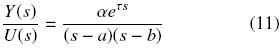
with a, b > 0 and assuming without loss of generality a > b. An observer based control strategy is proposed, which allows getting the estimation of the internal signals of the system, to be used as a control signal for the real process.
As a first step, the stability conditions for the controller and the observer are stated separately. These conditions will be used later to obtain the observer based controller closed loop stability conditions.
4.1 Controller scheme
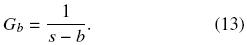
Now, let us introduce the proportional state feedback control strategy shown in the Fig. 2, where:
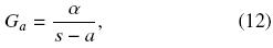
and
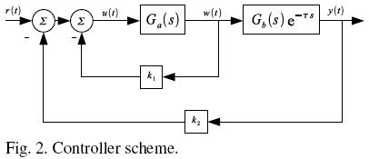
Lemma 3. Consider the delayed system (11) with the state feedback controller shown in Fig. 2. There exist constants k1 and k2 such that the closed–loop system is stable if and only if τ < b–1.
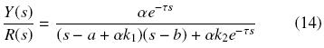
Proof. The aim of this proof is to apply Lemmas 1 and 2 to the closed loop system shown in the Fig. 2, with the following transfer function:
Let us consider αk1 > a. Then, we get a different system, only with one unstable pole, which can be stabilized under the stability condition given in Lemma 2, i.e., there exist constant gains k1 and k2 such that the closed–loop system is stable if and only if τ < b–1 –(αk1–a)–1. Now, as k1 can be as large as we wish, there exist proportional gains k1 and k2 such that the closed–loop system is stable if and only τ < b–1.
Note that the root locus technique and frequency domain analysis can be used to compute proper constant gains k1 and k2 in order to stabilize the proportional state feedback scheme.
4.2 Observer scheme
In most of the practical applications, some of the state variables may not be measured and then the control scheme of Fig. 2 cannot be implemented. Thus, an observer scheme based on an output injection strategy, as the presented in Fig. 3, can be implemented. The stability of the scheme in Fig. 3 (and consequently the error convergence in the observer schema as we will see later) can be tackled as follows.
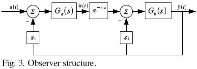
Lemma 4. Consider the delayed system (11), and the static output injection scheme shown in Fig. 3. There exist constants g1 and g2 such that the closed–loop system is stable if and only if τ < a–1.
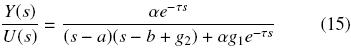
Proof. Consider the delayed system with the static output injection scheme shown in Fig. 3. The closed loop transfer function of the delayed system can be described as:
As in the controller structure, the purpose of the proof is to apply the conditions stated in Lemmas 1 and 2 to the observer scheme shown in the Fig. 3. First, consider g2 > b, thus, we get a system with only one unstable pole, which can be stabilized under the condition given in Lemma 2, i.e., considering the delayed system (5), and the static output injection scheme shown in Fig. 3, there exist constants g1 and g2 such that the closed–loop system is stable if and only if τ < a–1 – (g2 – b)–1.
As g2 can be as large as we wish, then we can conclude that τ < a–1.
4.3 Observer–based controller
Now, the proposed observer based controller is presented in Fig. 4, where the observer allows estimating the internal variable w(t) to be used in state feedback controller. It is important to note that, in the proposed scheme, only four proportional gains are enough to get a stable closed loop behavior. As a consequence of the previous results, the following lemma can be stated.
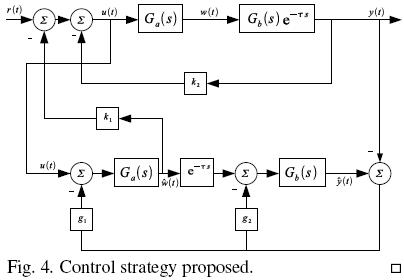
Lemma 5. Consider the observer based controller scheme shown in Fig. 4 and the time delay system given by Eq. (11). There exist gains k1, k2, g1 and g2 such that the closed–loop system is stable if and only if τ < a–1.
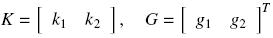
Proof. As a first step, in order to ensure an accurate estimation of the internal variables, let us demonstrate that the error signal converges asymptotically to zero, i.e.,  if and only if τ < a–1. Consider the state space representation of the system (11) characterized by the following equation:
with x(t) = [w(t)x2(t)]T and where:
Note that the state space representation characterized by (16) can be returned to its transfer function representation by mean of:
The dynamics of the estimated states and the control law can be described as follows

where  (t) is the estimated state of x(t) and the proportional gains are defined by:
Let e(t) := (t) – x(t), then we have:

Noting xe = [x(t) e(t)]T , and after a simple manipulation of variables we have the following closed loop system with the observer and the controller proposed in the Fig. 4:
It is easy to see that the observer and the controller can be designed separately, i.e. it satisfies the separation principle. Hence, the stability of the observer scheme is enough to assure the error convergence, i.e., there exist proportional gains g1 and g2 such that if and only if τ < a–1.
Then, considering the fact that the observer and controller can be designed independently and reminding the stability conditions stated previously in Lemma 3 and Lemma 4, it is clear that the observer stability condition is more restrictive than the controller stability condition, i.e., a–1 < b–1. Therefore, there exist k1, k2, g1 and g2 such that the closed–loop system is stable if and only if τ < a–1.
5 Second order unstable systems with a stable zero plus time delay
5.1 Controller scheme
Considering the unstable system given by Eq. (5) and the controller structure shown in Fig. 2, with:
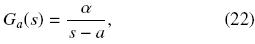
and
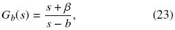
the stability conditions for the controller scheme are introduced below.
Lemma 6. Consider the delayed system (5), and the state feedback controller shown in Fig. 2. There exist constants k1 and k2 such that the closed–loop system is stable if and only if τ < b–1.
Proof. As in the Section 4, the objective of the proof is to apply the results of Lemma 1 to the following closed loop system transfer function
Let us choose k1 = (β + α)/α, then we obtain the following equivalent system:
Hence, it is possible to attach the stability conditions of Lemma 1, i.e., there exist constant gains k1 and k2 such that the closed–loop system is stable if and only if τ < b–1.
5.2 Observer scheme
First, let us consider the following modification to the static output injection scheme shown in Fig. 3, concerning the output injection to the subsystem Gb(s). Thus, we can state the following Lemma.
Lemma 7. Consider the delayed system (5), and the static output injection scheme shown in Fig. 3 (considering the modification shown in Fig. 5). There exist constants gains g1 and g2 such that the closed–loop system is stable if and only if τ < a–1.
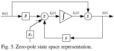
Proof. Consider the transfer function of the output injection scheme shown in Fig. 3, with Gb given by Eq. (23).
Let us choose g2 = β + b then we obtain the following equivalent system:
Hence, it is possible to attach the stability conditions of Lemma 1, i.e., there exist constant gains g1 and g2 such that the closed–loop system is stable if and only if τ < a–1.
5.3 Observer–based controller
Finally, the closed loop stability conditions for the observer–controller structure shown in the Fig. 4, with the sub–systems Ga(s) and Gb(s) given by eqs. (22)–(23) are stated in the incoming Lemma.
Lemma 8. Consider the observer based controller scheme shown in Fig. 4 and the time delay system (5). There exist constants k1, k2, g1 and g2 such that the closed–loop system is stable if and only if τ < a–1.
A complete proof can be done based in the state space representation of the closed loop system (21). Therefore, as the control structure holds the separation principle, i.e., the controller and the observer can be designed independently; it is easy to conclude that there exist k1, k2, g1 and g2 such that the closed–loop system is stable if and only if τ < a–1.
6 Numerical examples
The following examples are introduced in order to illustrate the performance of the control strategy proposed in this work.
Example 1. Consider the following second order unstable system plus time delay:
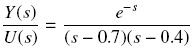
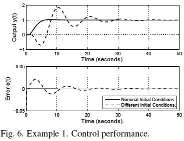
For this example without zeros, we have a = 0.7, b = 0.4, τ = 1 and α = 1. It is clear, since τ = 1 < α–1 = 1.4826, that the stability condition given in Lemma 5 is satisfied.
The following procedure is proposed in order to design the controller structure. To ensure the existence of a proportional gain k2 such that the closed loop system is stable, from Lemma 3 we get:
Let us choose k1 = 50.7, and then with a frequency domain analysis, it is possible to compute the proportional gain k2. For this example, 20 < k2 < 64.93. For the design of the observer, a very similar procedure is implemented. From Lemma 4 we get:
Let us choose g2 = 204.4, then by mean of a frequency domain analysis it is possible to compute the proportional gain g1 . For this example, 14 < g1 < 21.55.
Hence, the proportional gains computed for this example are k1 = 50.7, k2 = 30, g1 = 18 and g2 = 20.4. Fig. 6 illustrates the performance of the observer–based controller for a step reference in numerical simulations; the output y(t) and the error e(t) = ŷ(t) – y(t), are shown respectively. The continuous line indicates the output of the closed loop system with identical initial conditions between y(t) and ŷ(t). The dashed line point to the system performance whit different initial conditions (y(0) – ŷ(0) = 0.2).
Example 2. Chemical reactors often have significant heat effects, so it is important to be able to add or remove heat from them. In a jacketed CSTR (continuously stirred tank reactor) the heat is added or removed by virtue of the temperature difference between a jacket fluid and the reactor fluid. Often, the heat transfer fluid is pumped through agitation nozzles that circulate the fluid through the jacket at high velocity, as is shown in Fig. 7.
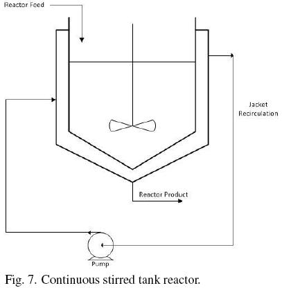
The following example has been tacked from Bequette (2003), and some parameters of the CSTR were changed in order to find an adequate model to apply the control strategy proposed in the present work. Here we consider a CSTR carrying out the simple reaction A  B. The balance on component A is
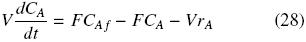
where CA is the concentration of component A in the reactor and rA is the rate of reaction per unit volume. The Arrhenius expression is normally used for the rate of reaction. A first order reaction results in the following
where k0 is the frequency factor, Ea is the activation energy, R is the ideal gas constant, and T is the reactor temperature on an absolute scale. The reactor energy balance, assuming constant volume, heat capacity (cp) and density (ρ), and neglecting changes in the kinetic and potential energy is
where –ΔH is the heat of the reaction, U is the heat transfer coefficient, A is the heat transfer area, Tf is the feed temperature, and Tj is the jacket temperature.
The parameter values of the system are given as Ea = 32,400 Btu/lbmol, k0 = 16.96 × 10¹² hr–1, –ΔH = 39,000 Btu/lbmol, U = 75 Btu/hr ft2°F, ρcp = 53.25 Btu/ft3°F. The operating values of the reactor are given by A = 309 ft2, CA f = 0.132 lbmol/ft3, Tf = 60°F, the operating volume V = 500 ft3 and the flow rate F = 300 ft3/hr. A steady state operating point is CA = 0.066 lbmol/ft3 and T = 101.1°F. Let consider the jacket temperature as the manipulated variable and the temperature of the CSTR as the controlled variable. Linearization around this steady state operating point yields the following transfer function model (by assuming a measurement time delay of 0.15 hr).
For the current example, the parameters of the system are a = 3.74, b = 0.2, β = 4.59, α = 0.87 and τ = 0.15. It is clear, sinceT = 0.15 < a–1 = 0.267, that the stability condition given in Lemma 7 is satisfied.
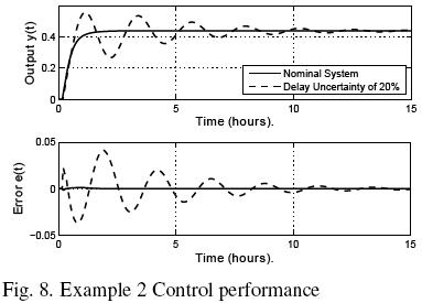
Hence, from Lemmas 6 and 7, for the proposed control strategy the proportional gains computed for this example are k1 = 9.57, k2 = 2.5, g1 = 5 and g2 = 4.79. Figure 8 illustrates the performance of the observer–based controller for a unit step reference in numerical simulations; the output y(t) and the error signals are shown respectively. The continuous line denotes the performance for the nominal system. The dashed line suggests the performance for the system whit an uncertainty in the delay operator of 20 %. The method performs well for nominal conditions as well as for the uncertain process.
Conclusions
A simple observer based controller is proposed in this work in order to stabilize second order unstable systems with two unstable poles, one "stable" zero plus time delay. Necessary and sufficient conditions are stated in order to guarantee the stability of the proposed schema. Therefore, only the model of the process and four proportional gains are enough to obtain a stable behavior of the closed loop system.
The procedure for the computation of the constant gains is quite easy and can be realized by mean a frequency domain analysis. The performance reached for the control structure proposed is shown by mean of numerical simulations, where it can be seen that some robustness is present in the control strategy under different initial conditions and for uncertainty in the delay term.
References
Bequette, B.W. (2003). Process Control. Modelling, Design and Simulation. Prentice Hall. [ Links ]
Del Muro, B., González, O.A. and Pedraza, Y.A. (2009). Stabilization of high order systems with delay using a predictor schema. IEEE 52nd International Midwest Symposium on Circuits and Systems, (pp. 337–340). Cancun. [ Links ]
del–Muro–Cuellar, B., Velasco–Villa, M., Jiménez–Ramírez, O., Fernández–Anaya, G. and Álvarez–Ramírez, J. (2007). Observer–based Smith prediction scheme for unstable plus time delay processes. Industrial & Engineering Chemistry Research 46(12), 4906–4913. [ Links ]
Gu, K., Kharitonov, V. L. and Chen, J. (2003). Stability of Time–Delay Systems. Birkhauser. [ Links ]
Malakhovski, E. and Mirkin, L. (2006). On Stability of Second–order Quasi–polynomials with a Single Delay. Automatica 42(6), 1041–1047. [ Links ]
Márquez, J., Del Muro, B., Velasco, M. and Álvarez, J. (2010). Control based in an observer scheme for first–order systems with delay. Revista Mexicana de Ingeniería Química 9(1), 43–52. [ Links ]
Niculescu, S.–I. (2001). Delay Effects on Stability: A Robust Control Approach (Vol. 269). Londres, Springer. [ Links ]
Normey–Rico, J.E. and Camacho, E.F. (2008). Dead–time compensators: A survey. Control Engineering Practice 16(4), 407–428. [ Links ]
Normey–Rico, J.E. and Camacho, E.F. (2009). Unified approach for robust dead–time compesator Design. Journal of Process Control 19, 38–47. [ Links ]
Palmor, Z.J. (1996). Time delay compensation Smith predictor and its modifications. The Control Hand–Book. CRC press, 224–237 [ Links ]
Rao, A.S. and Chidambaram, M. (2006). Enhanced two–degrees–of–freedom control strategy for second–order unstable processes with time delay. Industrial and Engineering Chemistry Research 45(10), 3604–3614. [ Links ]
Rao, A.S., Rao, V.S. and Chidambaram, M. (2007). Simple analytical design of modified Smith predictor with improved performance for unstable first–order plus time delay (FOPTD) processes. Industrial and Engineering Chemistry Research 46(13), 4561–4571. [ Links ]
Richard, J.P. (2003). Time–delay systems:an overview of some recent advances and open problems. Automatica 39, 1667–1694. [ Links ]
Shamsuzzoha, M., Jeon, J. and Lee, M. (2007). Improved analytical PID controller design for the second order unstable process with time delay. Computer Aided Chemical Engineering 24, 901–906. [ Links ]
Silva, G. J., Datta, A. and Bhattachaiyy, S. (2004). PID Controllers for Time–Delay Systems. Birkhauser. [ Links ]
Skogestad, S. (2004). Simple analytic rules for model reduction and PID controller tunning. Modeling, identification and Control 25, 291–309. [ Links ]
Smith, O.J. (1957). Close control of loops with dead time. Chemical Engineeering Progress 53, 217–219. [ Links ]
Zhong, Q.–C. (2006). Robust Control of Time–Delay Systems. Springer. [ Links ]

