


 text new page (beta)
 English (pdf)
 Article in xml format
 Article references
 Send this article by e-mail
 Cited by SciELO
  Similars in
SciELO
Similars in
SciELO 
 Permalink
Introduction
In recent years, the rise of unmanned aerial vehicles (UAV) has had a great impact on society so the area of possible applications increases continuously, for example: in the field of the military, trade, the search, rescue, dangerous environment monitoring, product delivery, as well as others (Floreano & Wood, 2015; Gupta et al., 2013; Cárdenas, 2015; Gutiérrez et al., 2017.
One of the main problems, when is generating a control system for an aerial vehicle, is to develop a dynamic model that describes the real behavior of the aircraft in the most precise way possible and at the same time; keep the model simple to design, analyze and investigate various control strategies, signal filtering, as well as implement the controller and filtering system in a digital system in a simple way. The quadcopter mathematical model is a set of equations that allows representing in detail the dynamic behavior of the quadcopter in flight; one of the main ways to approximate the dynamic model is applying the Euler-Lagrange methodology, which consists in observing the angular velocities of the vehicle, from a reference frame, movable but aligned to an inertial frame (Sadr et al., 2014; Rodríguez et al., 2016; Balasubramanian & Vasantharaj, 2013; Nonami et al., 2010; Beard & McLain, 2012; Garcia et al., 2006; Castillo et al., 2007; Carrillo et al., 2012; Raffo, 2007), this methodology incorporates the inertial and gyroscopic effects of the aircraft structure into the model. On the other hand, there is a model developed using Newton-Euler, which observes the angular velocities of the quadrotor from a mobile frame defined in the center of rotation of the aircraft (Bouabdallah & Siegwart, 2007; Falconi & Melchiorri, 2012; Elruby et al., 2012; de Jesus Rubio et al., 2014; Paiva, 2016; Bouabdallah & Siegwart, 2004; Hossain et al., 2010; Patete & Erazo, 2016; Agho, 2017), in this model, it is common to observe that the gyroscopic and inertial effects of the aircraft structure are despised, however, the gyroscopic effect of the rotation of the propellers is incorporated. Also, there are linear approximations, in which the flight dynamics around an operating point are frequently approximated (Sabatino, 2015; Roldan, 2016; Sevilla, 2014).
The implementation of the controller to stabilize the rotational movements of the quadrotor requires knowledge of the angular positions and speeds, these variables can be known through sensors or estimated through the model that describes the dynamics of the system. A methodology that allows fusing such data is the Kalman filter, this methodology has been used in countless areas of engineering since its proposal by Kalman (1960), particularly in the area of unmanned aerial vehicles; the main application is the estimation of the position and orientation of the aircraft (attitude) (You et al., 2020;. Bauer & Bokor, 2008; Loianno et al., 2016; Markley, 2003; Emran et al., 2015; Sanz et al., 2014; Sebesta & Boizot, 2013; Muñoz et al., 2013; Gośliński et al., 2013; Sarim et al., 2015; Tailanián et al., 2014; Amoozgar et al., 2013; Xiong & Zheng, 2015). Likewise, there are proposals for filtering signals in unmanned aircraft based on state observers, with the advantage of reducing the computational cost, due not processing the calculation at each moment the profit matrix or Kalman matrix (Escobedo et al., 2018; Macdonald et al., 2014; Hanley & Bretl, 2016; Lendek et al., 2011; Shi et al., 2018; Yu et al., 2015). Other proposals for filtering signals with a low computational cost include complementary filters (Noordin et al., 2018; Jung & Tsiotras, 2007; Euston et al., 2008; Yoo et al., 2001), however; these proposals are less efficient than observers or the Kalman filter.
In this work, the Euler-Lagrange model of a quadcopter is analyzed, such as proposed in (Beard & McLain, 2012; Garcia et al., 2006; Castillo et al., 2007; Carrillo et al., 2012; Raffo, 2007), but additionally incorporates the gyroscopic effects of the rotation of the helices, then approximations based on Taylor series are made, that simplify the model rotation dynamics which we called complete and allow us to represent the dynamics in a reduced non-linear model similar to the one proposed in (Bouabdallah & Siegwart, 2007; Falconi & Melchiorri, 2012; Elruby et al., 2012; de Jesus Rubio et al., 2014), additionally, a linear model is obtained.
Aircraft modeling
This section describes the model that defines the dynamic behavior of translation and rotation of the quadcopter. To develop this model, the Euler-Lagrange formalism is used.
Quadcopter speeds, forces and motions
Figure 1 shows the reference frames used
for modeling, as well as the free-body diagram. The orientation of the aircraft
is defined by the Euler angles:
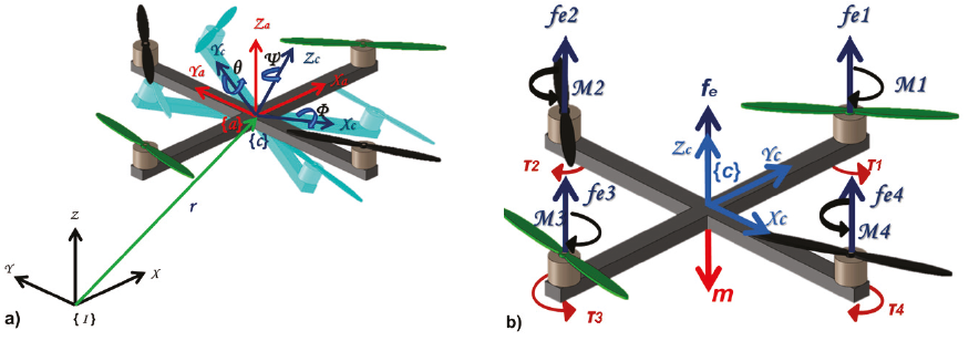
The total angular velocity of the aircraft is a sum of the rotational speeds in each reference axis of the system {c}. Therefore, the total angular velocity of the quadrotor represented by (p, q, r) =(Ω), is seen in the axes (X,Y,Z) of the reference frame {a} and is expressed according to the following relation (in the region where the Euler angles are valid), (Beard & McLain, 2012; Garcia et al., 2006; Castillo et al., 2007; Carrillo et al., 2012; Raffo, 2007).
According to Figure1b, the thrust force seen in the reference frame {c} is defined:
The thrust force fei for each engine and the aerodynamic drag force τi , which opposes the torque Mi generated by the rotation of the propellers, are expressed respectively, as:
Where, ωi is the angular velocity of each engine, ka and ke are positive definite constants that depend on the density of the air, the radius of rotation, the area and the shape of the propeller blades, as well as other factors. In conditions where the angular speed ωi of the motor is constant or the rates of change of this speed are small, the aerodynamic drag torque is equivalent to the torque produced by the motor (Beard & McLain, 2012; Garcia et al., 2006).
The thrust force acts on the “z” axis of the reference frame {c}, so the lift force in the inertial reference frame is defined:
The rotational movements are proposed on the bisector of the aircraft arms, that is, a flight in the "x" configuration. Then the rotation of an angle Φ (pitch) , is caused by a difference in the forces, such that:
The rotation of an angle θ (roll) , is achieved through a difference in the forces, which produces a torque:
To obtain a rotation of an angle ψ (yaw) it is achieved by a difference in the torques (T3 + T1) and (T2 + T4) which produces:
The aerodynamic drag torque Ti is expressed as:
Where fri is the force perpendicular to length l and kr relates fei and fri, so that equation (13) can be rewritten as:
Also, each engine-propeller pair is considered as a rigid disk rotating with a
speed ωi, around the “z”, axis, of the reference
frame {c}, so the following gyroscopic effects
The equations that define the relation of the total thrust force, the torques and the thrust forces of each engine, are given by equations (9), (10), (11), (12) and (13), then the forces in each engine as a function of the control inputs are:
Translation and rotation model
Due to the rotational kinetic energy and the translational kinetic energy do not have dependent terms; it is possible to separate the translation and rotation equations (Beard & McLain, 2012; Garcia et al., 2006; Castillo et al., 2007; Carrillo et al., 2012; Raffo, 2007). According to the Euler-Lagrange equations, the translation model is stated as:
Likewise, the dynamic model that describes the rotation of the quadcopter is given as:
Where
In turn, the Coriolis matrix is defined as (Castillo et al., 2007; Raffo, 2007):
Where:
Reductions and simplifications to the complete rotation model
In this section, two approaches to the rotation model are presented. Initially, a classical approximate linearization is approached, then, an approximation is presented to obtain a reduced non-linear model.
Linear model
To linearize the system, the rotation model is expressed in state variables and the zero equilibrium state is considered. The dynamics of rotation in state variables from (17) is expressed as:
The state vector and the equilibrium input vector, corresponding to:
Defining the incremental states and incremental inputs as:
Then the linearized system around an equilibrium point takes the form:
Where:
Therefore, the approximate linear system is defined by the following expression:
Simplifying the previous expressions, we obtain:
Reduced non-linear model
Another way to reduce the complexity of the model is to consider small movements,
that is, the transformation matrix
Then, applying these approximations to the inertia matrix (18) and Coriolis matrix (19), we obtain:
Then replacing (27), (28), (29) in (17) and rearranging, we obtain the reduced non-linear model for the rotation dynamics:
Computer torque controller
The open-loop dynamics of the quadcopter is unstable, so it is necessary to apply a closed-loop control system. In this section, we propose a control system based on the computed torque technique (Reyes, 2011; Sira et al., 2005).
Control based on the full model
The controller designed using the full model is:
Where:
Introducing the control in (17) and simplifying is obtained:
The term ξ, are constant disturbances. Then the closed-loop dynamics that define the behavior of the quadcopter is:
When each of the previous expressions is derived, we can observe that the perturbations considered constant become zero, then the closed-loop stability can be analyzed through the characteristic polynomial, choosing positive definite values for Ka, Kb and Ki, such that Ka, Kb > ki; the system is stable.
Signal filtering
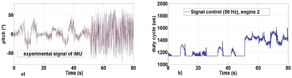
Figure 2a, shows the signal of one of the rotation angles of the quadcopter prototype, the signal is obtained from the projection of gravity on the axes of a low-cost Inertial Measurement Unit of 6 degrees of freedom (IMU 6 DOF, MPU6050), in addition, the angular positions and speeds of the drone can be accessed. Figure 2b shows one of the duty cycle signals (1000 us to 2000 us) with a frequency of 60 Hz, sent to the electronic speed controllers (ESC). From these graphs, we can observe the impact of mechanical vibration (noise) on the acquisition of the rotation signal, also, the noise increases as the speed of the motors increases.
For this reason, in this section, systems are developed and synthesized for filtering the quadcopter rotation signals.
Standard Kalman filter
The standard Kalman filter is an optimal state estimator and is applicable to a linear system, described by the following equation of state represented in discrete form; where: wk and vk are the process and measurement noise respectively.
The equations that describe the standard Kalman filter are defined as (Kalman, 1960; Simon, 2006):
Where:
yk = measurement matrix
Kk = filter gain matrix
Q = covariance of the noise process wk
R = covariance of the noise in the measurement vk
I = identity matrix
Also and according to the linear system (25), matrix A , matrix B , matrix C and the vector of states to be estimated are defined as:
Extended Kalman filter
The extended Kalman filter, unlike the standard KF, uses the non-linear model to estimate the system states. That is, the equation of state is represented as:
The equations that define the extended Kalman filter are (Simon, 2006):
The application of the previous equations requires the calculation of the matrices Ak and Ck, at each instant of time, these matrices are calculated trough the partial derivative of the equation of state and the output equation, then the results are evaluated in the vector of updated estimated states. According to the reduced nonlinear model (30), the matrix Ak and the matrix Ck are defined as:
Where:
|
|
|
|
|
|
|
|
|
|
|
|
|
|
|
|
|
|
|
|
Filter based on observer
The observability matrix of (A , C ), for the linear system (25), is full-range, so the state observer is established as:
The equation that defines the dynamics of the error that relates to the estimated states and the real states is:
We can verify the stability of the system through the eigenvalues of the matrix (A - koC), where the values can be chosen for the ko, matrix, such that, the observer behaves in a stable dynamic.
Filter based on extended observer
We can estimate the linear representation of the dynamics of the aircraft through a states observer, so the estimate states can be extrapolated to the non-linear model, that is, an extended Luenberger-type observer is proposed, now the estimation of the states is given by:
Now the dynamics of the error between the estimated states with the real states is defined as:
As the movements of the system are controlled around the equilibrium states
Simulation
In this section, numerical simulations in open-loop, closed-loop and filtering system are presented with the different models, the simulation was executed using MatLab software in the Simulink environment, the numerical method used was Runge-Kutta of fourth-order to a simulation step of 0.001s. The parameters that define the complete aircraft model, as well as the parameters used in the control and filtering system, are shown in Table 1.
Table 1: Model parameters
| Parameter | Value in model | Value in controller and filtering system |
Unit |
|---|---|---|---|
| l | 0.23 | 0.21 | m |
| d | 0.16 | 0.15 | M |
| m | 1.1 | 1.1 | Kg |
| g | 9.81 | 9.81 | m/s2 |
| Ix | 15x10-3 | 45x10-3 | Kg m2 |
| Iy | 15x10-3 | 45x10-3 | Kg m2 |
| Iz | 30x10-3 | 90x10-3 | Kg m2 |
| J | 1x10⁻⁴ | 3x10⁻⁴ | Kg m2 |
| kr | 1/12 | 1/10 | — |
| ke | 1.5x10⁻⁶ | 1.5x10⁻⁶ | — |
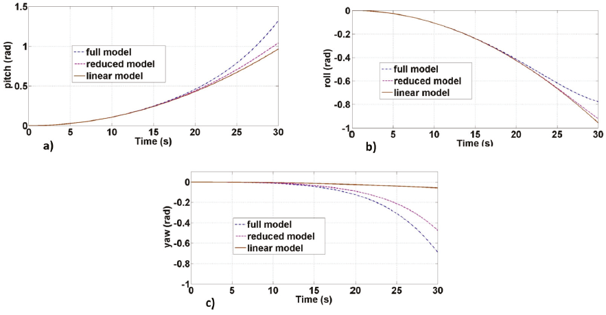
Open loop simulation
In open-loop simulations, the initial conditions are established as:
Control system simulation
In the closed-loop simulation, each of the controllers designed through the different models is applied to the complete non-linear dynamics of the rotation system, equation (17).
To compare the response of the different controllers; the performance index is
calculated under the
Figure 4 corresponds to the comparison of the response of the different controllers in the simultaneous movements in each axis of the aircraft. The overlapping responses of each controller are observed, only with the performance index presented in 4d, we can distinguish that the control designed with the reduced model offers the best performance.

Simulation of the control system and filtering system
Figure 5 illustrates through a block diagram the methodology used in the simulation of the noise process and filtering system. Table 2 defines the controller and observer gains.
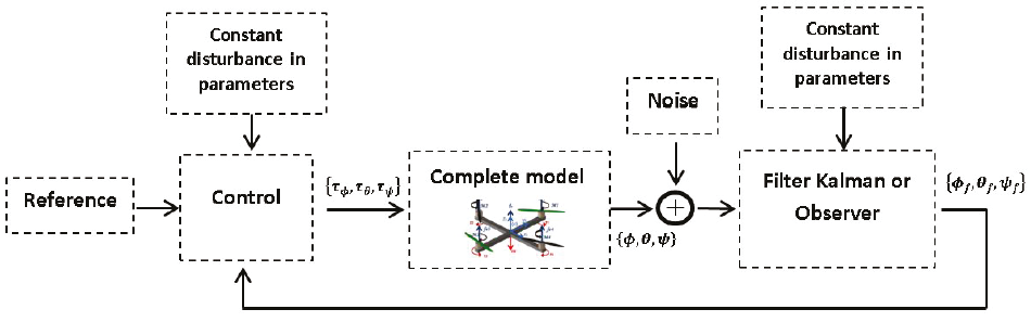
Table 2: Gains of the control system and filtering system
| Gains | |
|---|---|
|
|
|
|
|
|
Figures 6b to 6d, show the behavior with the reduced model in the filtering and control system for simultaneous movements in the axes of rotation of the aircraft, when is adding the white noise signal to the states of the system defined in 6a. The behavior of the reduced model offers the best performance for the controller and the filtering system as seen in Figure 7a and 7b. To obtain and compare the performance index of the control system, the different models are applied to the control and the filtering stage, then to obtain the performance index of the filtering stage, we proceed similarly.
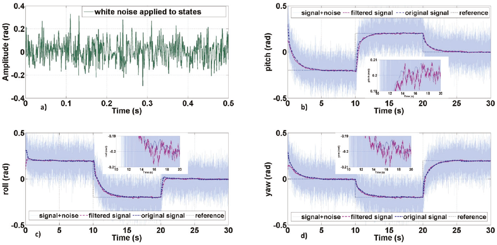
Figure 6: Response to the noise of the control system and filtering system with a reduced model, a) Noise added to the system states, b) pitch, c) roll, d) yaw
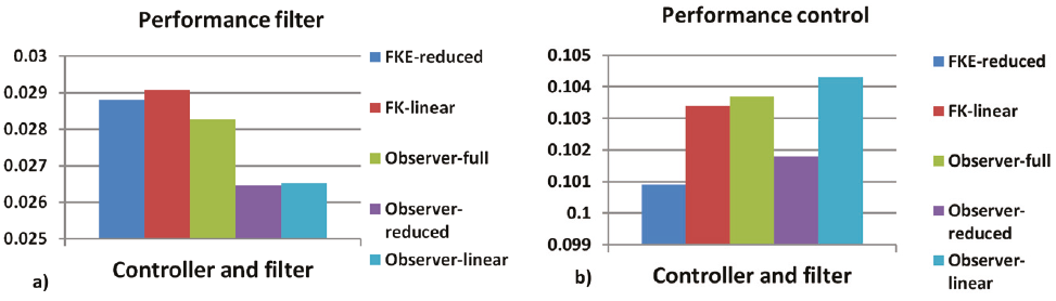
Figure 7: a) Control performance with different models and filters, b) filtering performance with different models and filters
We can see en Figure 7, that filter system with observers or Kalman filters is very similar, this can be explained because the operation of the aircraft is considered in a small region, even if there are combined movements in the rotations. Due to the implementation of the observer is simpler than the Kalman filter. Figure 8 shows the comparison of the controller and filtering through observers with the different models for combined or simultaneous movements in each axis of rotation.
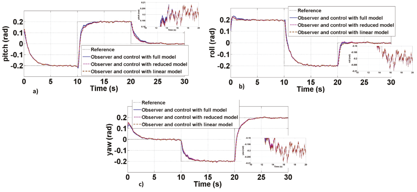
Figure 8: Comparison of the controller and filtering using observers with the different models for combined or simultaneous movements in each axis of rotation, a) Pitch angle, b) roll angle, c) yaw angle
It has shown that the performance offered by the control system and filtering system with the linear model is similar to that obtained with a Kalman filter or an observer using the full or reduced model. Due that it is simpler to implement a filtering and control system based on the linear model, we chose to implement the experimental part with this model.
Also, in order to compare the proposed control that bases its design on the approximate linear model of the aircraft with a control technique that does not require a dynamic model for its design, a comparison with a fuzzy logic controller is proposed.
Fuzzy logic control
The fuzzy-logic controller design is based, on producing changes in the control signal through the system error and its change reason, i.e. a PD system. The membership functions are presented in Figure 9. Where the following variables are defined for the error, its derivative, as well as the control or output signal; Negative Big (NB), Negative Small (NS), Zero (Z), Positive Small (PS) and Positive Big (PB).
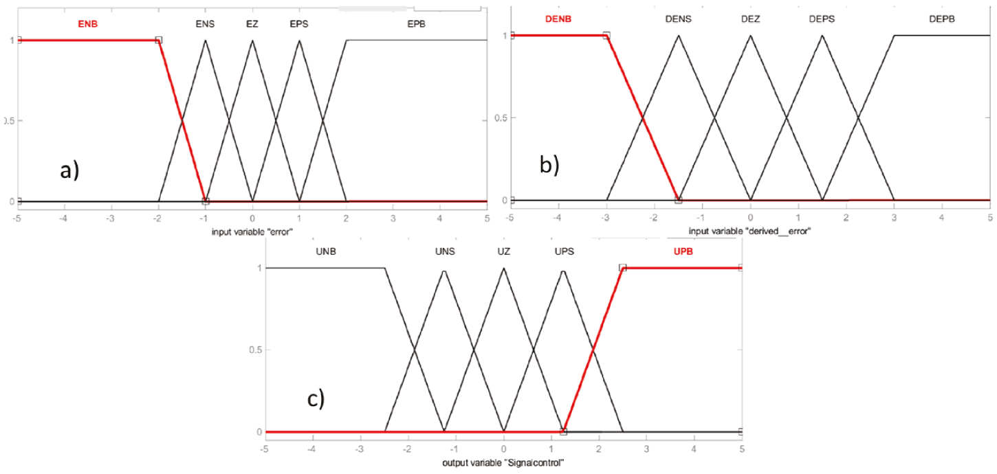
The inference rules are directly related to the linguistic variables defined in the membership functions and are presented in Table 3. Also, for the controller design and the defuzzification signals, the Fuzzy Logic Design toolbox from Matlab is used, establishing Sugeno's methodology and centroid defuzzification.
Table 3: Inference rules
| e(t) / d e(t)/dt | NB | NS | Z | PS | PB |
|---|---|---|---|---|---|
| NB | NB | NS | NS | NS | Z |
| NS | NS | NS | NS | Z | PS |
| Z | NS | NS | Z | PS | PS |
| PS | NS | Z | PS | PS | PS |
| PB | Z | PS | PS | PS | PB |
The comparison in a simulation of the proposed controller with the fuzzy controller is shown in Figure 10, as can be seen, any of the controllers achieves the objective of stabilizing the system with similar behavior, however, although the fuzzy controller offers adequate system behavior and not require a model for its design has the disadvantage; requires precise knowledge of the experimental behavior of the system to propose the membership functions and inference rules, likewise, the implementation in a microcontroller requires more computational resources for its execution, mainly in the defuzzification stage, therefore and due to that the behavior offered by the controller proposed as well as the relative simplicity with which it can be implemented in a microcontroller, it is chosen to implement the experimental part with this controller.
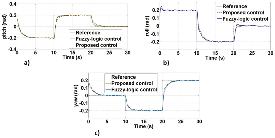
Figure 10: Comparison of the proposed controller and fuzzy-logic controller, a) Pitch angle, b) roll angle, c) yaw angle
Now the next section of the work shows the experimental results of this implementation.
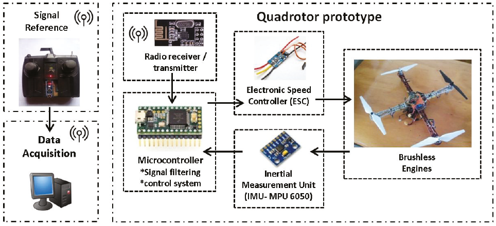
Microcontroller implementation and experimental results
The implementation is done according to the block diagram of Figure 11. The signals of the IMU are interpreted and filtered in the microcontroller, also the control signals are calculated using a linear model, the equations that define the linear observer are solved by the Runge Kutta numerical method at an operation step of 0.001s. The experimentation is divided into two stages. The first one, through a test bench that allows rotations in the aircraft's pitch, roll and yaw axes but restricts translational movements, the second stage in a quasi-static flight in which only the rotation movements are controlled around the origin and the translational movements of the aircraft are left free. Figure 12 shows both stages of experimentation.

Experimental results on the test bench
The experimental results of the implementation of the controller and filtering stage with the test bench are shown in Figure 13.
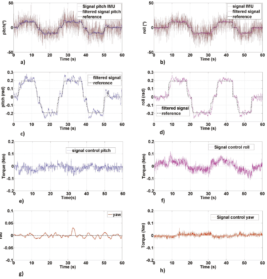
Figure 13: Results of the experimental stage on the test bench, a) Filtered signal for the pitch angle, b) filtered signal for the roll angle, c) trajectory tracking on the pitch axis, d) trajectory tracking on the roll axis, e) control signal for the pitch movement, f) control signal for the roll movement, g) yaw angle stabilization, h) control signal for the yaw movement
Experimental results in quasi-static flight
The experimental results of the implementation of the controller and filtering stage in a quasi-static flight are shown in Figure 14.
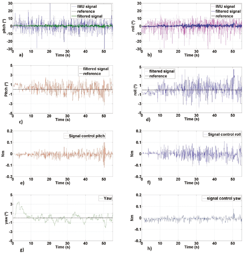
Figure 14: Experimental results of the quasi-static flight stage. a) Signal filtering for pitch angle, b) signal filtering for roll angle, c) pitch axis stabilization, d) roll axis stabilization, e) control signal for pitch movement, f) control signal for roll movement, g) yaw angle stabilization, h) control signal for the yaw movement
Conclusions
In this work, a dynamic model was developed using Euler-Lagrange for a quadcopter type aircraft, then a reduced model was obtained from the complete model, as well as a linear model. Afterward, its open-loop response was compared, observing that for an operating region less than 1 rad, the models behave similarly, later, controllers were designed using the computed torque technique based on the various models and a PID control, the controllers were compared through their performance index, it was determined that anyone controller achieves the objective of stabilizing or tracking the trajectory, later filtering systems were analyzed using observers and Kalman filters, where for each case the three analyzed models were applied, then it was compared the response of the controller and filtering system through a performance index when noise is added to the states and constant disturbances in the parameters, with this it was determined that a linear model is sufficient to design a controller and filtering system, which implies simple implementation and reduction of computational resources for operation with a microcontroller. Additionally, the proposed controller was compared in simulation with a fuzzy logic controller, it was observed that both controllers have similar behavior, however, the proposed controller is easy to implement in a microcontroller, and the stability of the system and filtering is justified with the mathematical analysis presented, against the fuzzy logic controller, for this reason, it was determined to implement the experimental part with said controller. Subsequently, the control and filtering system was implemented for a low-cost IMU and a 32-bit ARM microcontroller, the experimental results showed a behavior similar to the simulation, which validates the use of a linear model to stabilize and track trajectories in the operation of a non-aggressive or aerobatic flight of the aircraft. However, in the experimental part, it was noted that a linear model is sufficient to design the filter and controller, but a control strategy is necessary to give the system robustness to the disturbances caused by the wind or by the disturbances caused by no to know exactly the thrust force of each motor-propeller pair. It is also recommended to design an algorithm that allows improving the performance of the controller estimating the thrust forces of each motor.

