Gas path analysis

A physics-based model (thermodynamic model) constitutes the bases of one of the principal gas turbine diagnostic approaches called Gas Path Analysis (GPA). Using the model, the approach aims to estimate a health condition of each engine component.

At gas turbine steady states, engine gas path variables (fuel mass flow rate, thrust or power, gas path pressures and temperatures, etc.) depend on operating conditions (power set parameters and ambient conditions) and engine health parameters that determine actual component performance maps. Generally presented by a nonlinear physics-based static model, the relationship between the dependent variables (monitored variables) and the independent parameters is highly non-linear (^{Li, 2002}). The model is formed using gas path thermodynamic equations and conservation laws and is also called a thermodynamic model. Within the model, an (m×1)-vector Y→ of monitored variables is computed employing as arguments engine operational conditions joint in an (s×1)-vector U→ and engine health parameters united in an (r×1)-vector θ→. Given the above explanation, the thermodynamic model can be expressed by the following nonlinear dependency between the mentioned vectors (^{Urban, 1973}):

This physics-based model has many uses. First, it allows simulating many fault scenarios and creating a fault classification (^{Loboda et al., 2007}). Second, the model is the basis of GPA that involves nonlinear system identification techniques for the estimation of the parameters θ→ (^{Pinelli & Spina, 2002}). These techniques look for those parameters that provide the best tuning of the model to the measurements of a particular engine. Third, the thermodynamic model helps with forming many simplified models (^{Sampath & Singh, 2005}), like a linear model given by:

This static model is linearization of Eq. (1). A vector of fault parameters δθ→ presents relative changes of the health parameters induced by engine degradation, and a vector δU→ denotes relative changes of operating conditions. Matrixes H and G are constituted from influence coefficients for the corresponding fault parameters and operating conditions. Within a linear GPA, the use of the linear model makes it possible to estimate parameters δθ→ by simple analytical expressions, as proposed in (^{Urban, 1973}) upon the assumption of no variations in the operating conditions.

One can see in Eq. (2) that the mode of the influence on the monitored variables is the same for the fault parameters and the operating conditions i.e. through constant influence coefficients of the corresponding matrixes. Therefore, in addition to the matrix H, the matrix G may be a good indicator of the errors of the thermodynamic model, and we include the matrix G into our analysis as well.

Computation of influence coefficients

The fault influence matrix H is composed from the coefficients of the influence of small relative changes δθ→ on the respective changes of the monitored variables when operating conditions do not change. The matrix is usually calculated using the thermodynamic model given by Eq. (1). First, the monitored quantities Y→ are computed with nominal health parameters θ→0 corresponding to a healthy engine at a given operating point determined by a constant value of a power set variable. Small increase ∆θj is then added independently to each health parameter and the computation of Y→θJ0+∆θJ is made once more with the same power set variable value. Given the known values of a monitored variable Yi and a health parameter θj, the respective influence coefficient is finally calculated by:

This calculation is illustrated by Figure 1. As the variation ∆θj decreases, the coefficient Hij approaches the corresponding partial derivative.

Figure 1 Numerical calculation of the matrix H coefficients 

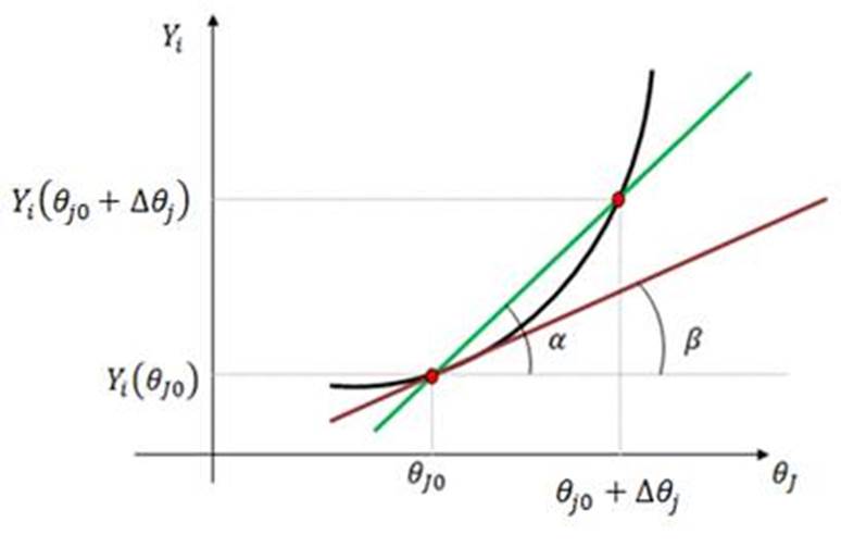
Having been computed, the influence coefficients constitute the [m×r]-matrix of fault influence as is shown below.

The accuracy of the matrix elements Hij computed according to Eq. (3) depends on variation value δθ _j. On the one hand, to reduce linearization errors, the variation value should be small. On the other hand, it should not be too small to avoid significant influence of the errors of numerical calculation of variables Y. For example, if δθ _j results in Yiθj-Yiθj0/Yiθj0=0.01 and numerical errors of Yiθj and Yiθj0 are equal to 10^-5, then an error of H_ij will be 2·10^-5/0.01=1.41·10^-3 i.e. 141 times greater than the error of Y. The above reasoning explains the need to look for the optimal variation value.

The matrix G in Eq. (2) presents the influence of operating conditions. This matrix is determined in the similar way as the matrix H. Its elements are calculated according to the following expression:

Once all the elements are computed, the [m×r]-matrix of operating condition influence takes the form:

Influence coefficient behavior and errors

^{Loboda et al. (2007)} have analyzed the behavior of the fault influence coefficients of an industrial power plant and an aircraft engine. Figure 2 illustrates this analysis by presenting the plots of different influence coefficients vs. operating points (steady states). As follows from Figure 2a, the level of the coefficients of the industrial power plant does not significantly change for different operating points, but there are some random perturbations in the coefficient behavior. For the aircraft engine presented in Figure 2b, it can be stated that some coefficients have a more significant general trend in the comparison with the power plant case, while the level of random perturbations is approximately the same, excepting the spike in point 26. However, this spike is caused by a normal opening of a compressor bypass valve and cannot be considered as a simulation error. The analysis of the thermodynamic models employed to compute the influence coefficients reveals that the random errors they mainly appear from not accurate enough approximation of engine component performances.

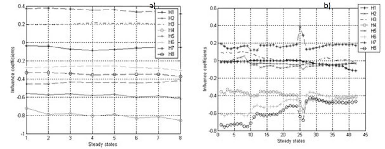
Figure 2 Fault influence coefficients versus steady states given by fuel consumption as a power set variable: a) coefficients of the influence of 8 fault parameters on the power turbine temperature of the industrial power plant; b) coefficients of the influence of 8 faults on the intermediate pressure turbine temperature of the aircraft engine (^{Loboda et al., 2007}) 

The analysis given in the rest of the present paper has the following purposes. First, it is necessary to ascertain whether the random fluctuations observed in Figure 1 are an intrinsic property of any thermodynamic model or they can be eliminated. Second, the matrix G is also a derivative matrix, and it is of practical interest to verify whether its coefficients have random errors. Third, some diagnostic methods are based on the assumption that changing operating condition do not significantly influence on influence coefficient values i.e. the impact of faults is not considerably affected by an engine regime. To the contrary, in multipoint algorithms a diagnostic accuracy is improved if the operating condition influence is significant. Therefore, in this paper a general dependence of influence coefficients from operating conditions will also be evaluated. To see all the details of the influence coefficient behavior, a graphical mode is very useful. To draw well-grounded and general conclusions, we will analyze plots of different elements of both influence matrices of two engines.

Analyzed quantities of test case engines

The models of a turboshaft and a turbofan of the GasTurb 12 software were selected to conduct the analysis of the matrices H and G. Table 1 specifies the quantities considered in both engines. These quantities determine the structure of the matrixes: turboshaft [8×6]-matrix H, turbofan [8×5]-matrix H, and [8×2]-matrixes G of both engines. During the matrixes computation, a spool speed (ZXN or ZXNH) is employed as a power set variable. In the section below, we will analyze the fault influence matrixes H of both engines. We firstly will find the optimal variation value for the fault parameters δθ, as well as the operating conditions U. The optimal value provides the highest accuracy of the corresponding matrix and linear model. Once the mentioned value is found, each influence matrix will be computed under different operating conditions, and the impact of the operating conditions on the behavior of the matrix elements will be estimated.

Optimal variation value of fault parameters

In order to find the optimal variation value of fault parameters, we computed matrixes H with different levels of the variation. The simulation was performed in GasTurb 12 with six fault parameters for the turboshaft and seven for the turbofan. First, a healthy engine (when δθ→=0) was simulated. Its performance is labeled as ''design point''. Then, many off design points were simulated when the engine model had different values of each fault parameter varying independently. In Figure 3 the mentioned points are shown in the compressor map of the turbo shaft.

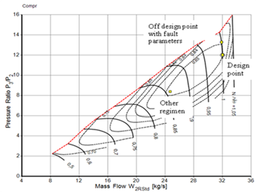
Figure 3 Design and off-design conditions during engine operation simulations by GasTurb 12 (^{GasTurb GmbH, 2015}) 

Conventionally, maximum value of 0.05 to 0.07 (5 to 7 %) is considered for the fault parameters (^{Fentaye et al., 2019}). For this reason, a total range of the variation was approximately limited by 0.1 for both engines. To better present the behavior of the influence coefficients, the range was divided into three intervals with individual variation increment in each one. In total, 285 variation values of each fault parameter were introduce one by one in the turboshaft model. The monitored variables and matrices H were computed for each value. For the turbofan, the number of considered variation values and the resulting matrices was 294.

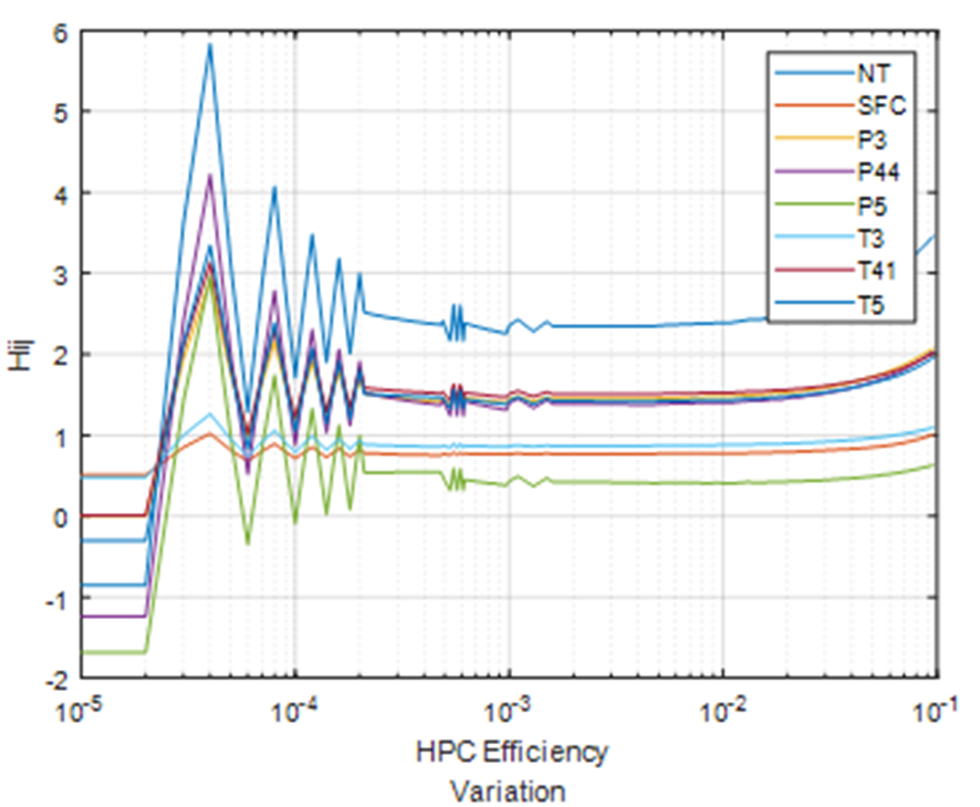
Table A1 of the Appendix section illustrates the set of variation values for the turboshaft and presents the corresponding influence coefficients of a compressor efficiency fault parameter. For this engine, Figure 4 shows the semi logarithmic graphs of the coefficients of influence of the same fault parameter on all the monitored variables (these coefficients constitute a column in the matrix H). According to the behavior of the coefficients, a total span of the fault parameter variation can be divided into four intervals. In the first interval, the fault parameter variations are too small, and the engine model of GasTurb 12 does not react to these variations. The second interval is characterized by significant random perturbations in the influence coefficients because of numerical errors of the simulation in GasTurb. In the third interval, the coefficients are practically constant. In the fourth interval, the coefficients begin to change significantly because of linearization errors. Given such a behavior of the coefficient, the third interval presents proper fault parameter variations. The other influence coefficients of the matrix H show similar behavior, and a common variation value 0.005 (0.5 %) was chosen for all fault parameters. All further calculations of the turboshaft matrix H use this value.

Figure 4 Selection of the optimal value of the compressor efficiency variation (turboshaft) 

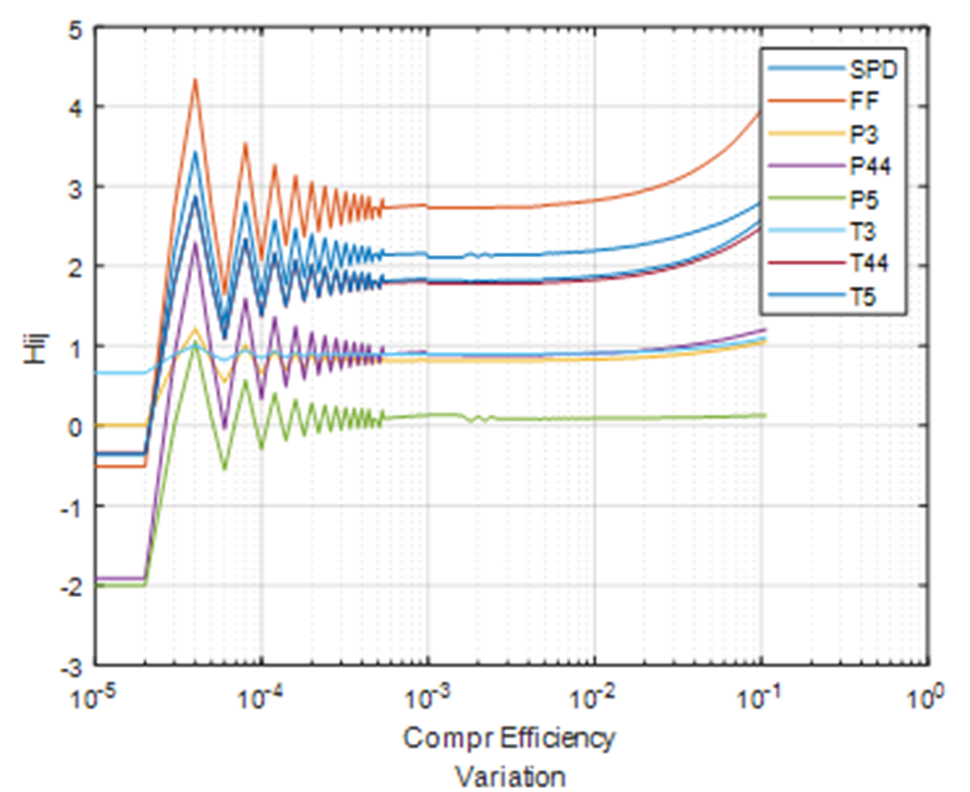
Figure 5 illustrates the behavior of the high pressure compressor efficiency influence coefficients of the turbofan engine. Comparing Figures 5 and 4, one can state that the influence coefficient plots of both engines are quite similar, and the variation value optimal for the turboshaft seems to be correct for the turbofan as well. The above graphical analysis of the variations was repeated for all fault parameters of both engines and the variation value 0.005 was found the best. Therefore, this value was used to determine all the matrixes H in the next subsection.

Figure 5 Selection optimal value of the HPC efficiency variation (turbofan) 

Influence of operating conditions on the matrix H

Once the optimal variation value was selected, we can compute the matrixes H of both engines. Computed at the design point, these matrices are given as an example in Table A2 of the Appendix.

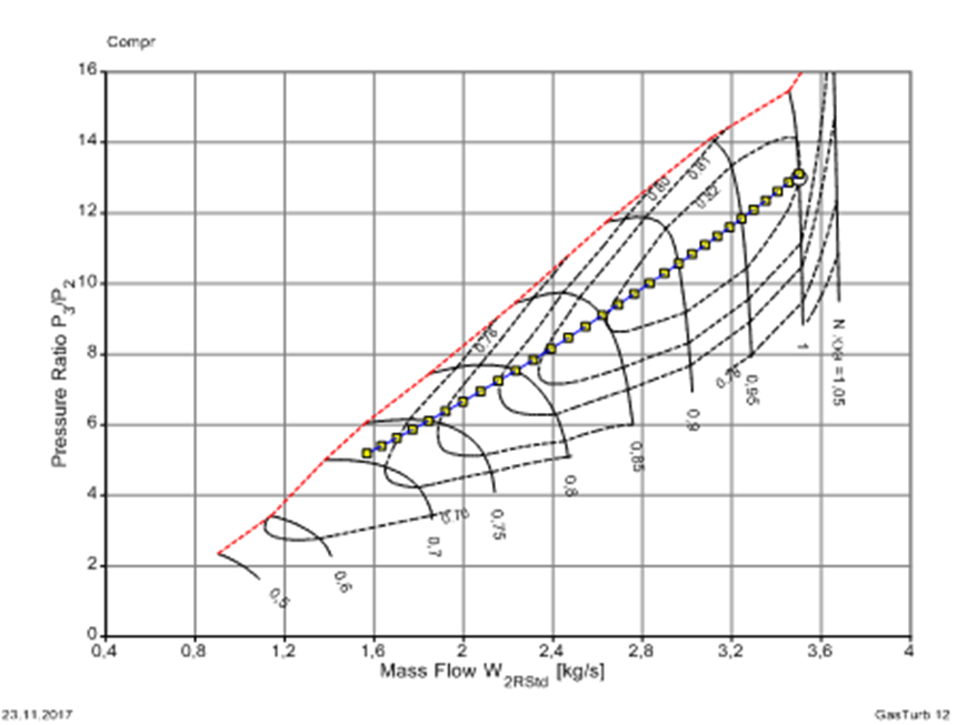
To analyze the influence of the operating conditions, many operating points were determined for each engine by independently changing the relative rotation speed of HPC (power set variable) from 1 to 0.72 and the ambient temperature in a range 264 to 312 K. Figure 6 shows on a turboshaft compressor map the simulated operating points with different rotation speed values. For each value of the speed or temperature, the fault influence matrix H was computed using a fixed variation 0.005 for each of the six fault parameters. Table A3 illustrates the set of the temperature values and the resulting turboshaft fault influence coefficients. Once the matrixes H were calculated under different operating conditions, we can plot the influence coefficients against each condition variable, HPC spool speed or ambient temperature, and analyze their behavior.

Figure 6 Turboshaft simulated operating points (^{GasTurb GmbH, 2015}) 

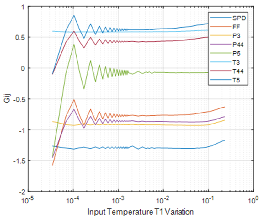
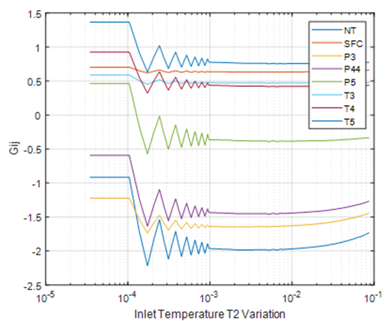
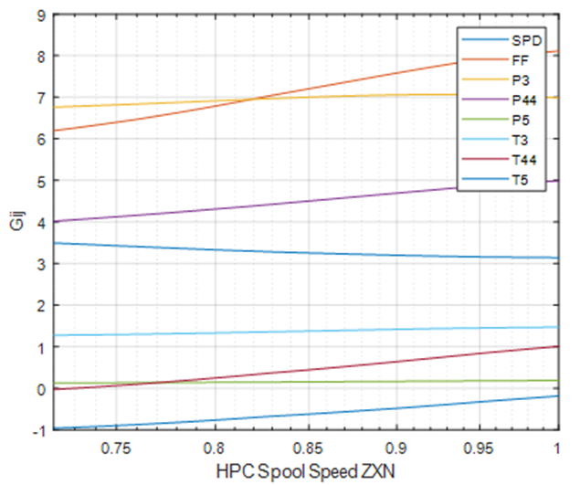
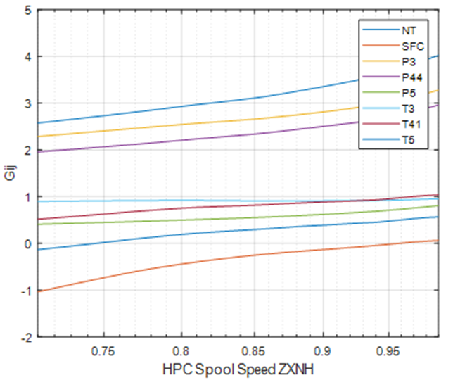
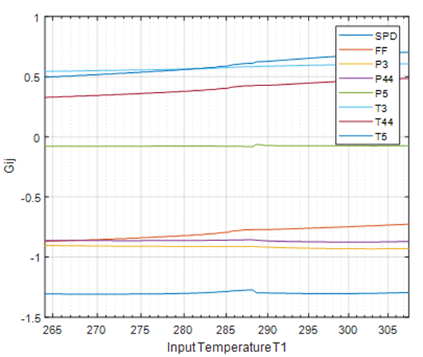
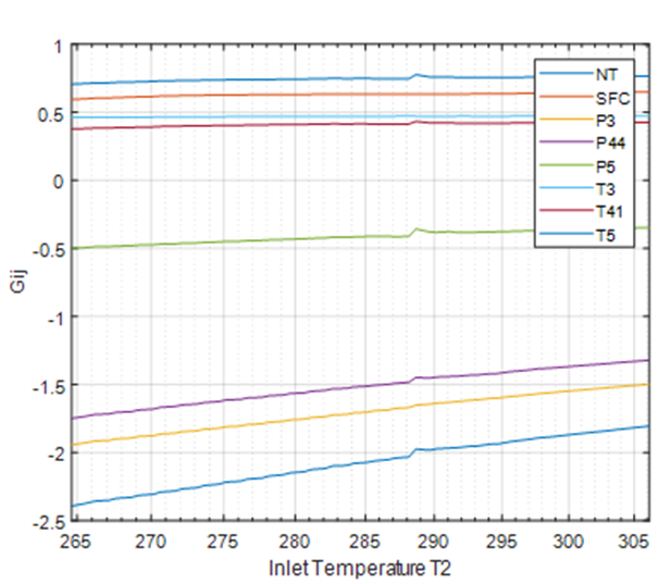
Figures 7, 8, 9 and 10 illustrate the behavior of the fault influence coefficients of both engines. As before, the influence coefficients of compressor efficiency are presented. They are plotted against each operating condition. Using the plots presented, let us firstly analyze possible random errors in the influence coefficients and then evaluate general trends in these coefficients. It can be seen in Figures 7 and 8 that the change of the HPC spool speed does not cause random point-to-point errors, and irregularities in the behavior of the influence coefficients are rare and small. As to Figures 9 and 10 where the input temperature varies, some low level random errors are observed in the right side of the figures. In general, all irregularities and errors are smaller than those in Figure 1, and the coefficients change more gradually.

Figure 7 Compressor efficiency influence coefficients vs HPC spool speed (turboshaft) 

Figure 8 Compressor efficiency influence coefficients vs input temperature (turboshaft) 

Figure 9 HPC efficiency influence coefficients vs HPC spool speed (turbofan) 

Figure 10 HPC efficiency influence coefficients vs input temperature (turbofan) 

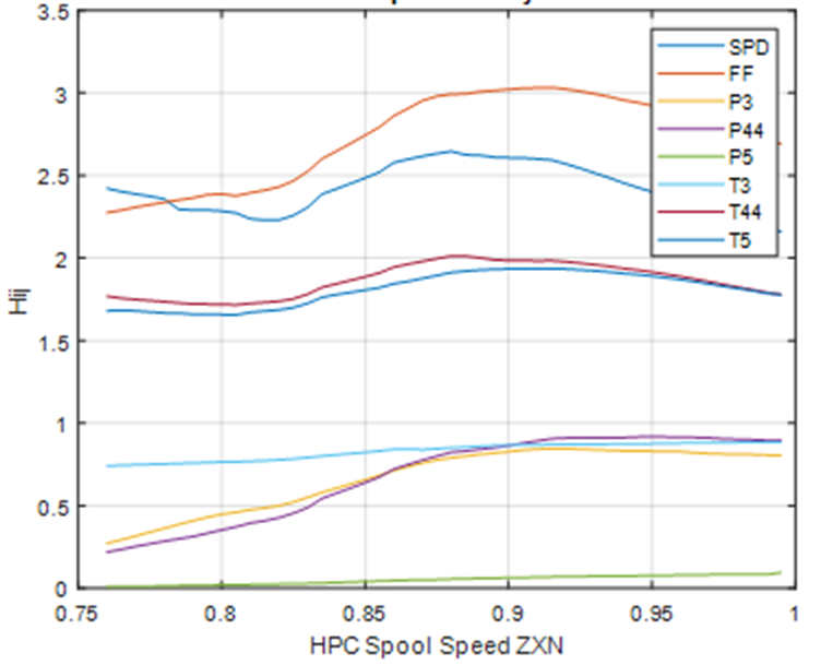
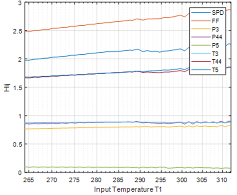
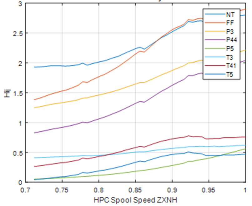
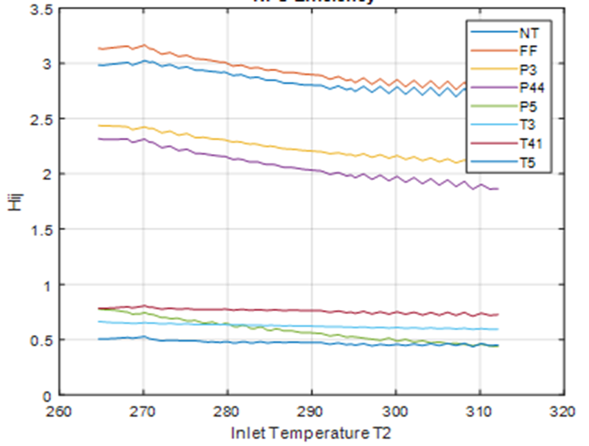
General behavior of the influence coefficients depends on a particular variable of operating conditions. The rotation speed has a significant impact. As is shown in Figures 7 and 9, the influences coefficients depend significantly on the speed for both engines, and this dependence is strongly nonlinear. For the turboshaft, the dependence has different directions: the coefficients mainly grow on left side of Figure 7 and their curves descend on the right side. In contrast, the turbofan coefficients constantly grow (Figure 9). As to the input temperature, Figures 8 and 10 show that its impact is by far lower, and the coefficients change lineally and slowly or remain constant.

The next section deals with the operating condition influence matrix G. As with the matrix H, the optimal variation value is determined first, and then the influence of operating conditions on this matrix is analyzed.

Optimal variation of operating conditions

The optimal value of the variation of operating conditions corresponds to the most accurate calculation of the matrix G. As with the matrix H, we compute the matrix G with different variation values and analyze the plots of the influence coefficients Gij against a variation value. These plots constructed for both engines are shown in Figures 11 and 12 for the HPC spool speed (first operating condition) and in Figures 13 and 14 for the input temperature (second operating condition). As before, we look for the intervals where the coefficients are constant and choose in this intervals the optimal variation value. By doing so for all of the matrix G coefficients, we selected the optimal value 0.005 that is used in all of the further calculations of the matrix G. Table A4 of the Appendix exemplifies the operating condition influence matrices by presenting the influence coefficients obtained at the design point.

Figure 11 Selection of the optimal variation value of HPC spool speed for the turboshaft 

Figure 12 Selection of the optimal variation value of HPC spool speed for the turbofan 

Figure 13 Optimal variation of input temperature for the turboshaft 

Figure 14 Optimal variation of input temperature for the turbofan 

Influence of operating conditions on the matrix G

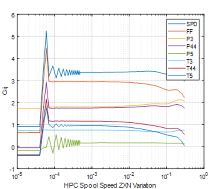
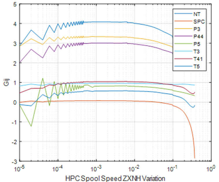
Figures 15 and 17 for the turboshaft and Figures 16 and 18 for the turbofan illustrate the behavior of the influence coefficients of the matrix G under varying operating conditions, a HPC spool speed and an engine input temperature. We can see in these figures that the coefficients behavior is gradual and does not manifest perturbations and random faults. Additionally, it follows from Figures 15 and 16 that the impact of the rotation speed is now small and lineal. In contrast, the input temperature variations cause now more significant and nonlinear changes of the coefficients.

Figure 15 Influence of HPC spool speed on the matrix G coefficients for the turboshaft 

Figure 16 Influence of HPC spool speed on the matrix G coefficients for the turbofan 

Figure 17 Influence of input temperature on the matrix G coefficients for the turboshaft 

Figure 18 Influence of the input temperature on the matrix G coefficients for the turbofan 

Summing up the results of sections 3 and 4, we can draw the following conclusions. First, random errors of the matrix H are rare and small, and they are practically absent in the calculation of the matrix G. Second, general changes of the matrixes H and G because of varying operating conditions can be significant. Third, when the operating conditions vary, the behavior of the coefficients of the matrixes H and G is quite different.