


 text new page (beta)
 English (pdf)
 Article in xml format
 Article references
 Send this article by e-mail
 Cited by SciELO
  Similars in
SciELO
Similars in
SciELO 
 Permalink
Introduction
Oil refineries are big energy-consuming industrial facilities (Rossi et al., 2020; Ulyev et al., 2018). Several authors, such as (Ocic, 2005), state that the equivalent energy consumption relative to the processed crude, ranges between 4 % and 8 % (Szklo & Schaeffer, 2007; Ochoa & Jobson, 2015) between 7 % and 15 %, and (Worrel et al., 2015), between 27 % and 35 % with data calculated by this agency. Therefore, energy consumption in an oil refinery may vary in time, due to the type of processed crude, the complexity of the refinery (U.S. Energy Information Administration, 2012), loading capacity, and other operational factors (Hui et al., 2016).
Additionally, the processes with a greater energy intensity in relation to a major load capacity are atmospheric distillation “AD”, vacuum distillation “VD”, catalytic reforming “CR”, catalytic cracking “CC”, hydrocracking “HC”, hydrotreatment “HT”, coking “CK”, and alkylation “AK” (Worrel et al., 2015). The energy consumption of AD and VD is 35 % and 45 % of the total of the different processes (Szklo & Schaeffer, 2007), and more than 80 % of the energy consumption results from the refinery products, including refinery gas (RG), petroleum coke (PC), liquid gas (LG), fuel oil (FO), and other refined products (Wang et al., 2004), which are used for direct heating or for vapor generation; additionally electricity (EL) is used to power pumps, compressors and other ancillary equipment (Worrel et al., 2015).
In recent years, the processed crude has become heavier and the established refineries have focused in procuring lighter fuels such as gasoline (Demirbas & Bamufleh, 2017). Among the different oil-derived products produced from an oil barrel in a United States refinery, 45 % to 48 % is gasoline (U.S. Energy Information Administration, 2019) and, according to (Wang et al., 2004), 53.7 % of the energy used in a particular refinery is used in the production of fuel.
In contrast, although refineries satisfy society’s energy demands, they can also affect air quality (Ragothaman & Anderson, 2017). The World Health Organization (WHO) has identified polluted air as the biggest health hazard and, thus, efforts are needed to maintain a good air quality (World Health Organization, 2020). This industry is responsible for the emission of several air pollutants (Kalabokas et al., 2001; Hadidi et al., 2016), emitting millions of tons (MM tons) to the air with a potential health risk (Wakefield, 2007). Some of the pollutants emitted by this industry include carbon monoxide (CO), particles (PM), nitrogen oxides (NOx), sulfur oxides (SOx), and volatile organic compounds (VOC) (Worrel et al., 2015).
To this date, Mexico has six oil refineries (Cadereyta, Madero, Minatitlán, Salamanca, Salina Cruz and Tula), which process three types of crude oils (Olmeca, Istmo and Maya), which are considered as super light, light, and heavy, respectively (Petróleos Mexicanos, 2018). According to the Energy Information System the six refineries had a gasoline production yield of 30.2 % in 2007 and 28.1 % in 2017 (Sistema de Información Energética, 2019).
According to data obtained from the National Institute of Transparency, Access to Information and Personal Data Protection (INAI), the Transformation Subsector of Petróleos Mexicanos (INAI, 2017), reported that the energy self-consumption of the Oil Refining Sector (SNR) was only fuel oil (FO) and electricity (EL), which represented 8 % of the equivalent energy relative to the total processed crude in 2007 and 9 % in 2016. Additionally. Mexico’s oil refineries emitted a total of 326,456 tonnes (tons) in 2016, with a proportion of 84 % (SOx), 6 % (NOx), 4 % (PM) and 5 % (VOC).
Finally Miranda (2018), published an informative note in the newspaper La Jornada, where it is mentioned that gasoline importation increased 63 % and production decreased 50 %, that is, Refining National System decreased from a production of 437,000 barrels per day (B/D) in 2013, to 217,000 B/D in the first half of 2018. On the other hand, the current situation limits fuel offer for the next years, implying that Mexico will continue importing gasoline.
In this sense, the set-up of the oil refining industry in Mexico has the main objective of satisfying the demand of different fuels, particularly of gasolines, consuming the greater volume of the crudes in the country and reporting clearly and timely the energy and environmental impact that this industry will have. However, this depends on a series of challenges which are the bases of study of the present paper, and which will be decisive in the fuel transformation processes.
The principal objective of this study is to estimate the energy consumption and the emissions of CO, SOx, NOx, PM and VOC of the Mexican oil refining industry for the year 2030, with the idea of contributing and extending new information on the atmospheric emissions of this industry, applying different refining technologies used to satisfy the gasoline demand.
Consequently, this paper, after the Introduction, begins with information on the possible gasoline demand scenarios in Mexico, after which the energy consumption and atmospheric emissions estimates are modeled. Finally, the last two sections emphasize and discuss its results and conclusions, respectively.
Gasoline demand scenarios in Mexico
In a paper published in (Bauer et al., 2003) examined the impact of the gasoline demand in Mexico, as a consequence of the increase in the number of vehicles which circulate when a certain per capita level is reached. Thus, the four scenarios in gasoline demand calculated by these authors are labeled as A, B, C and D in this paper. The first scenario (A) was based on the historical yearly car increase (4.3 %) for the period 1980-2000, and of 4 % for the period 2000-2030. Scenarios B, C and D were established considering a yearly increase in the average gross national product (GNP) of 3.7, 5.3 and 6.2 %, respectively (2000-2030), based on the Gompertz Curve to obtain the number of vehicles as a function of the per capita income and, in consequence, as a function of the year when such income is reached. In this way, the gasoline demand scenarios for the year 2030 established by the authors are: 1306000, 2142000, 2765000 and 2904000 B/D, respectively.
On the other hand, the Mexican Department of Energy (Secretaría de Energía, 2016) reported that the gasoline demand will have an average yearly increase of 1.9 % for the period 2016-2030, that is 834000 B/D to 1063000 B/D in 2030. Finally, a particular scenario was developed by performing a correlation Montecarlo simulation between the historical gasoline demand relative to the relevant macroeconomic indicators for this study (using the Crystal Ball program). These indicators are the currency exchange, the national consumer price index (NCPI), the GNP, the balance of trade and, additionally, the country’s population. A correlation analysis was performed for each of these and forming groups of indicators with the historical demand of gasoline. From this analysis one can conclude that it is convenient to relate the gasoline demand with the GNP, the NCPI and the population, since a better correlation (R2= 0.8395) was obtained with a fuel demand scenario of 1193000 B/D for the year 2030.
Modeling of the energy consumption and atmospheric emissions
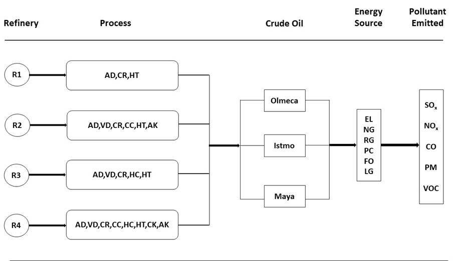
Different projections were determined by modeling four types of refineries (R1 “hydroskimming”, R2 “cracking”, R3 “hydrocracking” and R4 “full conversion”), three types of crudes (Olmeca, Istmo and Maya), and eight types of processes (AD “atmospheric distillation”, VD “vacuum distillation”, CR “catalytic reformation”, CC “catalytic cracking”, HC “hydrocracking”, HT “hydrotreatment”, CK “coking”, AK “alkilation”).
The steps for the modeling and estimation for the six energy sources (EL “electricity”, NG “natural gas”. RG “refinery gas”, PC “petroleum coke”, FO “fuel oil”, LG “liquid gas”) and five types of atmospheric pollutants (SOx “sulfur oxides”, NOx “nitrogen oxides”, CO “carbon monoxide”, PM “particles”, VOC “volatile organic compounds”) are then described:
Step 1. Required crude volume
This was calculated from the following equation:
Where:
µ = crude oil volume (B/D)
δ = gasoline demand (B/D)
P = current gasoline production (325000 B/D)
λ i,r = gasoline production yield (% vol.)
i = type of analyzed crude (Olmeca, Istmo, Maya)
r = type of refinery (R1, R2, R3, R4)
γ = production efficiency (100 %)
The data base required that feeds Equation 1 is given in Table 1 and 2.
Table 1 Gasoline demand scenarios (B/D)
| δ | |||||
|---|---|---|---|---|---|
| A | B | C | D | s | m* |
| 1,306,000 | 2,142,000 | 2,765,000 | 2,904,000 | 1,063,500 | 1,193,900 |
Source: (Bauer et al., 2003) (Secretaría de Energía, 2016)
Own elaboration
Table 2 Gasoline yield by type of crude oil and refinery analyzed (% Vol.)
| λ | ||||
|---|---|---|---|---|
| i | r | |||
| R1 | R2 | R3 | R4 | |
| Olmeca | 21.41 | 33.06 | 47.16 | 54.55 |
| Istmo | 18.51 | 29.97 | 39.78 | 55.23 |
| Maya | 15.30 | 23.00 | 33.43 | 54.57 |
Source: (Baird, 1996)
Step 2. Carrying capacity for each type of analyzed process
This was calculated from the following equation:
Where:
þ = carrying capacity (B/D)
µ = crude oil volume (B/D)
Ƭ j = operation rate (% Vol.)
j = process type (AD, VD, CR, CC, HC, HT, CK, AK)
The operation rates for the different types of analyzed processes are given in Table 3.
Table 3 Operating rate by type of crude and refinery analyzed (% Vol.)
| j | Olmeca | Istmo | Maya | |||||||||
|---|---|---|---|---|---|---|---|---|---|---|---|---|
| R1 | R2 | R3 | R4 | R1 | R2 | R3 | R4 | R1 | R2 | R3 | R4 | |
| AD | µ | |||||||||||
| T | ||||||||||||
| VD | ---- | 38 | 29 | 38 | ---- | 43 | 43 | 43 | ---- | 61 | 22 | 61 |
| CR | 19 | 17 | 31 | 23 | 16 | 15 | 27 | 28 | 14 | 15 | 19 | 32 |
| CC | ---- | 32 | ---- | 31 | ---- | 28 | ---- | 28 | ---- | 24 | ---- | 23 |
| HC | ---- | ---- | 16 | 6 | ---- | ---- | 13 | 8 | ---- | ---- | 8 | 11 |
| HT | 25 | 23 | 34 | 29 | 21 | 19 | 29 | 33 | 17 | 18 | 23 | 35 |
| CK | ---- | ---- | ---- | 4 | ---- | ---- | ---- | 15 | ---- | ---- | ---- | 32 |
| AK | ---- | 5 | ---- | 6 | ---- | 4 | ---- | 7 | ---- | 3 | ---- | 5 |
Source: (Baird, 1996)
Step 3. Energy consumption by type of process
Energy consumption was calculated using the following equation using the data base shown in Table 4:
Where:
£ = energy consumption in million British thermal units per day (MMBtu/D)
þ = carrying capacity (B/D)
Ɛe = specific ene/rgy (British thermal unit per barrel “Btu/B”)
e = minimum (x), maximum (y), average (z)
Table 4 Specific energy by type of process
| j | e | ||
|---|---|---|---|
| x | y | z | |
|
|
|
|
|
Source: Own elaboration based on (Pellegrino et al., 2007)
Step 4. Energy source consumed by type of process
The following equation is used:
Where:
Ƒ = energy consumption by energy source (MMBtu/D)
£ = energy consumption (MMBtu/D)
ƒ = energy source (%) (EL, NG, RG, PC, FO, GL)
j = process type (AD, VD, CR, CC, HC, HT, CK, AK)
Table 5 gives the energy percentage by type of analyzed source in percentage.
Table 5 Energy consumed by type of energy source and process analyzed (%)
| j | f | |||||
|---|---|---|---|---|---|---|
| EL | NG | RG | PC | FO | LG | |
| AD | 6.2 | 25.7 | 46.2 | 17 | 3.1 | 1.8 |
| VD | 3.9 | 26.3 | 47.2 | 17.4 | 3.2 | 2.00 |
| CR | 8.7 | 21 | 48.3 | 15.5 | 4.6 | 1.8 |
| CC | 12.5 | 5.5 | 10 | 70.9 | 0.7 | 0.4 |
| HC | 49.9 | 13.7 | 24.6 | 9.1 | 1.7 | 1 |
| HT | 47.9 | 14.2 | 25.6 | 9.5 | 1.8 | 1 |
| CK | 23 | 21.1 | 37.9 | 14 | 2.5 | 1.4 |
| AK | 37.6 | 17.1 | 30.7 | 11.3 | 2.1 | 1.3 |
Source: Own elaboration based on (Pellegrino et al., 2007)
Step 5. Emissions estimations
The following equation is used as indicated by the United States Environmental Protection Agency (U.S. Environmental Protection Agency, 2020)
Where:
E = emission of each type of pollutant (tons per day “tons/D”)
Ƒ = energy consumption by energy source (MMBtu/D)
cƒ = emission factor of each type of pollutant (tons/MMBtu)
c = pollutant (SOx, NOx, CO, PM, VOC)
ƒ = energy source (EL, NG, RG, PC, FO, GL)
Table 6 gives the emission factor of each type of pollutant in tons/MMBtu
Table 6 Emission factors by type of energy source
| f | c f | ||||
|---|---|---|---|---|---|
| SOx | NOx | CO | PT | COV | |
| EL | 6.6E-04 | 2.5E-04 | 3.2E-05 | 1.8E-04 | 1.8E-06 |
| NG | 6.4E-05 | 3.7E-05 | 1.4E-06 | 2.7E-06 | |
| RG | 6.4E-05 | 3.7E-05 | 1.4E-06 | 2.7E-06 | |
| PC | 1.1E-03 | 4.3E-04 | 1.1E-05 | 3.3E-04 | 2.3E-06 |
| FO | 7.7E-04 | 1.2E-04 | 1.6E-05 | 2.0E-05 | 2.5E-06 |
| LG | 9.4E-05 | 3.7E-05 | 3.2E-06 | 2.7E-06 | |
Source: Own elaboration based on (Pellegrino et al., 2007)
Finally, Equation 6 summarizes the matrix that was used to estimate the total emission estimates by type of analyzed crude and refinery.
Where:
Ʌ = total emissions of pollutants (tons/D)
i = type of analyzed crude (Olmeca, Istmo, Maya)
r = type of refinery (R1, R2, R3, R4)
Ƒ = energy consumption by energy source (MMBtu/D)
c ƒ = emission factor of each type of pollutant (tons/MMBtu)
j = process type (AD, VD, CR, CC, HC, HT, CK, AK)
Figure 1 shows the block diagram for determining energy consumption and atmospheric emissions, considering the type of refining technology.
Results and discussion
Figure 2 shows the volume of processed crude for the projections PA, PB, PC, PD, Ps and Pm, required to satisfy the gasoline demand for the year 2030.
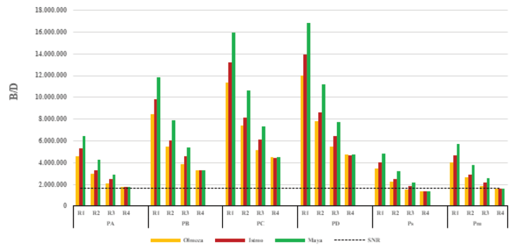
The figure clearly shows how the required crude volumes for three of the six projections exceeds, by much, the planned volumes that will be sent to the national refinery system NRS (SENER, 2016) (dotted line). Only the scenario based on the vehicular growth tendency (PA), the one suggested by the Mexican Department of Energy (Ps), and the one modeled by the Montecarlo program (Pm), almost completely agree for a very complex refinery (R4) and for the three types of crude.
Table 7 shows the carrying capacity for the different processes which are a function of the carrying capacity that feeds the DA process for each refinery and type of crude analyzed.
Table 7 Carrying capacity (B/D)
| Proceso | OLMECA | ISTMO | MAYA | |||||||||
|---|---|---|---|---|---|---|---|---|---|---|---|---|
| R1 | R2 | R3 | R4 | R1 | R2 | R3 | R4 | R1 | R2 | R3 | R4 | |
| PA | ||||||||||||
| VD | ---- | 1,134,708 | 612,397 | 687,689 | ---- | 1,415,036 | 1,066,079 | 767,855 | ---- | 2,586,001 | 652,953 | 1,089,940 |
| CR | 877,677 | 508,601 | 636,527 | 416,660 | 868,007 | 480,091 | 664,579 | 497,782 | 877,706 | 622,295 | 568,381 | 569,131 |
| CC | ---- | 952,810 | ---- | 555,277 | ---- | 926,009 | ---- | 492,045 | ---- | 1,032,183 | ---- | 417,136 |
| HC | ---- | ---- | 340,334 | 112,882 | ---- | ---- | 324,731 | 148,917 | ---- | ---- | 224,547 | 192,119 |
| HT | 1,134,267 | 674,771 | 708,105 | 517,367 | 1,123,990 | 638,190 | 724,554 | 583,573 | 1,081,601 | 757,929 | 661,698 | 626,298 |
| CK | ---- | ---- | ---- | 74,038 | ---- | ---- | ---- | 265,366 | ---- | ---- | ---- | 575,747 |
| AK | ---- | 157,061 | ---- | 114,051 | ---- | 138,590 | ---- | 123,251 | ---- | 113,071 | ---- | 95,673 |
| PB | ||||||||||||
| VD | ---- | 2,101,696 | 1,134,277 | 1,273,732 | ---- | 2,620,918 | 1,974,583 | 1,422,215 | ---- | 4,789,770 | 1,209,395 | 2,018,778 |
| CR | 1,625,625 | 942,026 | 1,178,969 | 771,734 | 1,607,716 | 889,221 | 1,230,928 | 921,989 | 1,625,681 | 1,152,610 | 1,052,751 | 1,054,140 |
| CC | ---- | 1,764,787 | ---- | 1,028,479 | ---- | 1,715,146 | ---- | 911,362 | ---- | 1,911,800 | ---- | 772,616 |
| HC | ---- | ---- | 630,363 | 209,080 | ---- | ---- | 601,464 | 275,823 | ---- | ---- | 415,904 | 355,842 |
| HT | 2,100,880 | 1,249,806 | 1,311,546 | 958,263 | 2,081,844 | 1,182,050 | 1,342,013 | 1,080,890 | 2,003,332 | 1,403,830 | 1,225,592 | 1,160,023 |
| CK | ---- | ---- | ---- | 137,133 | ---- | ---- | ---- | 491,508 | ---- | ---- | ---- | 1,066,393 |
| AK | ---- | 290,907 | ---- | 211,245 | ---- | 256,696 | ---- | 228,285 | ---- | 209,429 | ---- | 177,205 |
| PC | ||||||||||||
| VD | ---- | 2,822,311 | 1,523,189 | 1,710,460 | ---- | 3,519,560 | 2,651,614 | 1,909,853 | ---- | 6,432,052 | 1,624,063 | 2,710,962 |
| CR | 2,183,008 | 1,265,021 | 1,583,206 | 1,036,340 | 2,158,958 | 1,194,110 | 1,652,980 | 1,238,113 | 2,183,082 | 1,547,809 | 1,413,711 | 1,415,576 |
| CC | ---- | 2,369,885 | ---- | 1,381,116 | ---- | 2,303,223 | ---- | 1,223,844 | ---- | 2,567,304 | ---- | 1,037,525 |
| HC | ---- | ---- | 846,498 | 280,768 | ---- | ---- | 807,690 | 370,396 | ---- | ---- | 558,507 | 477,850 |
| HT | 2,821,214 | 1,678,330 | 1,761,239 | 1,286,826 | 2,795,652 | 1,587,343 | 1,802,153 | 1,451,497 | 2,690,220 | 1,885,165 | 1,645,814 | 1,557,764 |
| CK | ---- | ---- | ---- | 184,152 | ---- | ---- | ---- | 660,033 | ---- | ---- | ---- | 1,432,030 |
| AK | ---- | 390,651 | ---- | 283,675 | ---- | 344,710 | ---- | 306,557 | ---- | 281,237 | ---- | 237,964 |
| PD | ||||||||||||
| VD | ---- | 2,983,090 | 1,609,961 | 1,807,900 | ---- | 3,720,059 | 2,802,669 | 2,018,652 | ---- | 6,798,468 | 1,716,582 | 2,865,398 |
| CR | 2,307,368 | 1,337,086 | 1,673,397 | 1,095,378 | 2,281,948 | 1,262,135 | 1,747,146 | 1,308,645 | 2,307,446 | 1,635,983 | 1,494,246 | 1,496,217 |
| CC | ---- | 2,504,891 | ---- | 1,459,794 | ---- | 2,434,431 | ---- | 1,293,563 | ---- | 2,713,557 | ---- | 1,096,630 |
| HC | ---- | ---- | 894,721 | 296,762 | ---- | ---- | 853,702 | 391,496 | ---- | ---- | 590,323 | 505,072 |
| HT | 2,981,931 | 1,773,940 | 1,861,572 | 1,360,133 | 2,954,913 | 1,677,770 | 1,904,816 | 1,534,185 | 2,843,474 | 1,992,558 | 1,739,571 | 1,646,505 |
| CK | ---- | ---- | ---- | 194,642 | ---- | ---- | ---- | 697,633 | ---- | ---- | ---- | 1,513,609 |
| AK | ---- | 412,905 | ---- | 299,835 | ---- | 364,347 | ---- | 324,021 | ---- | 297,258 | ---- | 251,520 |
| Ps | ||||||||||||
| VD | ---- | 854,790 | 461,327 | 518,045 | ---- | 1,065,965 | 803,091 | 578,435 | ---- | 1,948,068 | 491,878 | 821,066 |
| CR | 661,165 | 383,136 | 479,504 | 313,875 | 653,881 | 361,659 | 500,636 | 374,986 | 661,188 | 468,783 | 428,169 | 428,734 |
| CC | ---- | 717,764 | ---- | 418,297 | ---- | 697,575 | ---- | 370,664 | ---- | 777,557 | ---- | 314,234 |
| HC | ---- | ---- | 256,378 | 85,036 | ---- | ---- | 244,624 | 112,181 | ---- | ---- | 169,154 | 144,726 |
| HT | 854,458 | 508,314 | 533,424 | 389,740 | 846,716 | 480,757 | 545,816 | 439,613 | 814,784 | 570,958 | 498,466 | 471,798 |
| CK | ---- | ---- | ---- | 55,774 | ---- | ---- | ---- | 199,903 | ---- | ---- | ---- | 433,717 |
| AK | ---- | 118,316 | ---- | 85,916 | ---- | 104,402 | ---- | 92,847 | ---- | 85,178 | ---- | 72,072 |
| Pm | ||||||||||||
| VD | ---- | 1,005,087 | 542,441 | 609,133 | ---- | 1,253,393 | 944,298 | 680,141 | ---- | 2,290,596 | 578,365 | 965,434 |
| CR | 777,417 | 450,502 | 563,815 | 369,064 | 768,853 | 425,249 | 588,663 | 440,920 | 777,444 | 551,209 | 503,454 | 504,118 |
| CC | ---- | 843,969 | ---- | 491,846 | ---- | 820,229 | ---- | 435,838 | ---- | 914,274 | ---- | 369,486 |
| HC | ---- | ---- | 301,457 | 99,988 | ---- | ---- | 287,636 | 131,906 | ---- | ---- | 198,897 | 170,173 |
| HT | 1,004,697 | 597,691 | 627,216 | 458,267 | 995,594 | 565,288 | 641,787 | 516,910 | 958,047 | 671,349 | 586,111 | 554,754 |
| CK | ---- | ---- | ---- | 65,581 | ---- | ---- | ---- | 235,052 | ---- | ---- | ---- | 509,978 |
| AK | ---- | 139,119 | ---- | 101,023 | ---- | 122,759 | ---- | 109,172 | ---- | 100,155 | ---- | 84,744 |
Based on Table 7, the carrying capacity minima and maxima for the different analyzed processes are obtained when using one type of refinery and crude as follows: VD (R3-olmeca, R2-maya), CR (R4-olmeca, R1-maya), CC (R4-maya, R2-maya), HC (R4-olmeca, R3-olmeca), HT (R4-olmeca, R1-olmeca), CK (R4-olmeca, R4-maya) and AK (R4-maya, R2-olmeca).
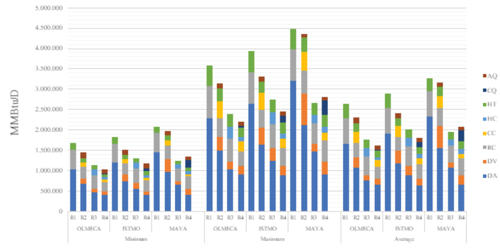
With the idea of reducing the presentation of the results obtained in this study, only the highest projections (PD) are presented below.
Figure 3 show at first glance, it can be seen that the process that uses the most energy is atmospheric distillation (AD) regardless of the type of analyzed projection. It can also be seen that, regardless of the minima, maxima or average values, the use of Maya crude implies a higher energy consumption in very complex refineries (R4) relative to the complex ones (R3).
In this same sense Figure 4 show type of energy consumed considering an average consumption
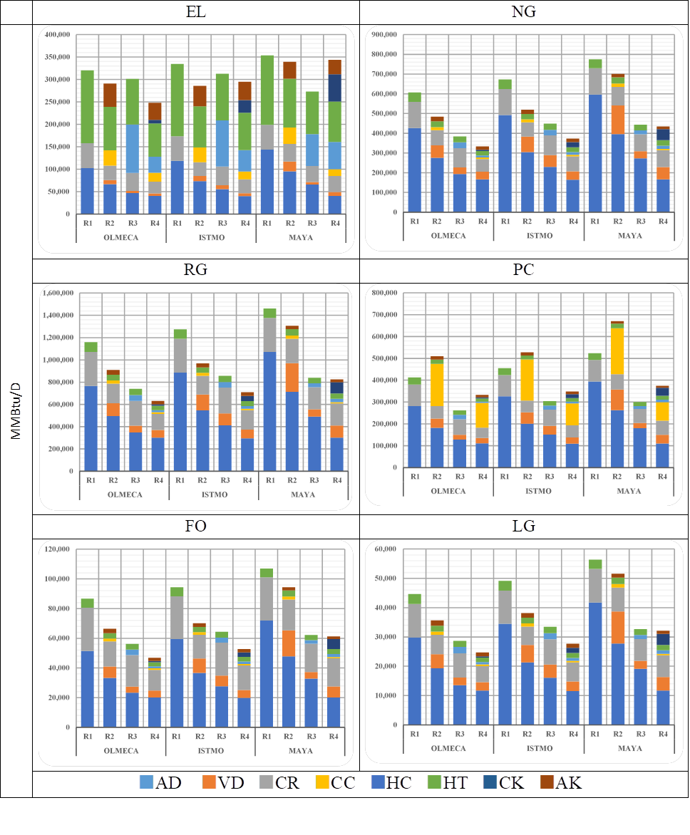
From Figure 4, it can be appreciated that both liquid gas (LG) and fuel oil (FO) are sources with the least energy requirement to satisfy the gasoline demand. Most of the energy consumption occurs both for atmospheric distillation (AD) and catalytic reforming (CR). For CR, the difference in energy consumption between the different types of refineries is not great, in contrast with AD, where energy consumption practically triplicates when a simple refinery is used (R1) when compared to a very complex one (R4). The percentage increase between these two types of refineries is progressive as the crude becomes heavier. On the other hand, and in the context of atmospheric distillation, the use of LG and fuel oil in a complex refinery (R3) consumes between 7-18 %, 28-43 %, and 57-64 % more energy than in a very complex refinery (R4), if Olmeca, Istmo and Maya crudes are refined.
Figure 5 show the emissions by type of analyzed pollutant for three energy sources (EL, FO and RG) at the different types of refineries, types of crudes and processes studied, considering an energy consumption average.
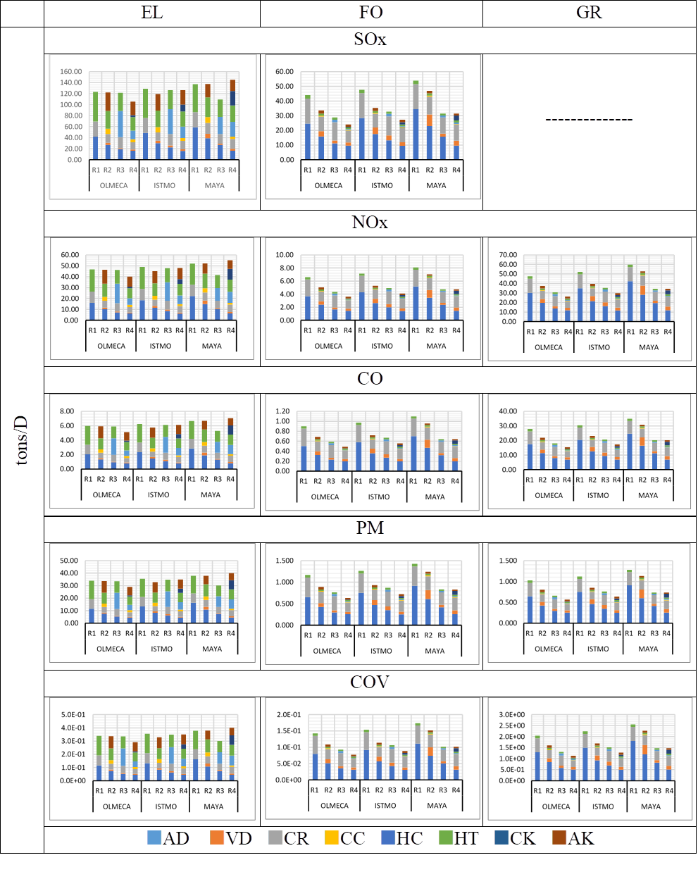
Figure 5 shows that fuel oil (FO) generates the least emissions when used as a heat source in the refineries. In contrast, refinery gas (RG) is comparable only in total particles (PM). The use of electricity as an energy source for refineries implies and emission of up to 3, 6, 7, 33, and 2.5 times more SOx, NOx, CO, PM and VOC, respectively. On the other hand, the use of refinery gas (RG) implies the emission of 7, 33 and 15 times more NOx, CO and VOC, respectively. The proportion of emitted pollutants varies according to the three used sources of energy.
Figure 6 gives the total emissions of the analyzed pollutants considering an average energy consumption for each type of refinery and crude oil for the different projections in the study.
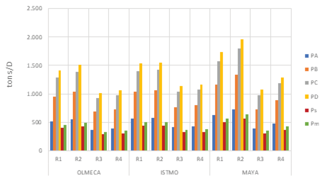
In Figure 6 it can be seen that regardless of the analyzed projection, refinery R3 processing Olmeca crude has the lower emissions and that R2 processing Maya crude has the highest, with a difference, in ton/day, of 350 for PA, 648 (PB), 870 (PC), 952 (PD), 273 (Ps) and 310 (Pm).
Table 8 shows the energy consumption relative to the total consumption by refinery type and crude processed, for a minimum consumption, an average and a maximum consumption.
Table 8 Energy consumption relative to the total consumption (percentage)
| Proceso | OLMECA | ISTMO | MAYA | |||||||||
|---|---|---|---|---|---|---|---|---|---|---|---|---|
| R1 | R2 | R3 | R4 | R1 | R2 | R3 | R4 | R1 | R2 | R3 | R4 | |
| Minimum | ||||||||||||
| DA | 61.3% | 46.2% | 40.9% | 39.0% | 64.9% | 48.8% | 42.7% | 34.2% | 69.1% | 48.8% | 52.9% | 30.2% |
| DV | ---- | 9.8% | 6.7% | 8.3% | ---- | 11.7% | 10.2% | 8.2% | ---- | 16.4% | 6.5% | 10.2% |
| RC | 28.7% | 19.3% | 30.5% | 22.1% | 26.0% | 17.5% | 28.1% | 23.4% | 23.1% | 17.4% | 25.0% | 23.4% |
| CC | ---- | 8.2% | ---- | 6.7% | ---- | 7.7% | ---- | 5.3% | ---- | 6.6% | ---- | 3.9% |
| HC | ---- | ---- | 12.6% | 4.6% | ---- | ---- | 10.6% | 5.5% | ---- | ---- | 7.6% | 6.1% |
| HT | 10.1% | 7.0% | 9.3% | 7.5% | 9.2% | 6.3% | 8.4% | 7.5% | 7.8% | 5.8% | 7.9% | 7.0% |
| CQ | ---- | ---- | ---- | 2.2% | ---- | ---- | ---- | 6.8% | ---- | ---- | ---- | 13.0% |
| AQ | ---- | 9.5% | ---- | 9.6% | ---- | 8.0% | ---- | 9.2% | ---- | 5.0% | ---- | 6.2% |
| Average | ||||||||||||
| DA | 62.9% | 46.7% | 42.4% | 40.2% | 66.5% | 49.1% | 44.1% | 35.5% | 70.7% | 48.7% | 54.3% | 31.3% |
| DV | ---- | 10.5% | 7.3% | 9.0% | ---- | 12.4% | 11.2% | 9.0% | ---- | 17.3% | 7.1% | 11.1% |
| RC | 24.1% | 16.0% | 26.0% | 18.6% | 21.8% | 14.4% | 23.8% | 19.9% | 19.4% | 14.2% | 21.0% | 19.8% |
| CC | ---- | 11.9% | ---- | 9.8% | ---- | 11.0% | ---- | 7.8% | ---- | 9.4% | ---- | 5.8% |
| HC | ---- | ---- | 12.2% | 4.4% | ---- | ---- | 10.2% | 5.3% | ---- | ---- | 7.3% | 5.9% |
| HT | 13.0% | 8.9% | 12.0% | 9.6% | 11.8% | 8.0% | 10.8% | 9.7% | 9.9% | 7.2% | 10.2% | 9.1% |
| CQ | ---- | ---- | ---- | 2.1% | ---- | ---- | ---- | 6.8% | ---- | ---- | ---- | 12.8% |
| AQ | ---- | 6.1% | ---- | 6.2% | ---- | 5.1% | ---- | 6.0% | ---- | 3.2% | ---- | 4.1% |
| Maximum | ||||||||||||
| DA | 63.8% | 47.0% | 43.2% | 40.7% | 67.3% | 49.2% | 44.7% | 36.1% | 71.5% | 48.7% | 55.1% | 31.9% |
| DV | ---- | 10.9% | 7.7% | 9.4% | ---- | 12.9% | 11.7% | 9.4% | ---- | 17.8% | 7.4% | 11.7% |
| RC | 22.0% | 14.5% | 23.8% | 17.0% | 19.8% | 13.0% | 21.7% | 18.2% | 17.6% | 12.8% | 19.2% | 18.2% |
| CC | ---- | 13.6% | ---- | 11.3% | ---- | 12.5% | ---- | 9.0% | ---- | 10.6% | ---- | 6.7% |
| HC | ---- | ---- | 12.0% | 4.3% | ---- | ---- | 10.0% | 5.2% | ---- | ---- | 7.2% | 5.8% |
| HT | 14.2% | 9.6% | 13.2% | 10.5% | 12.8% | 8.6% | 11.8% | 10.7% | 10.9% | 7.8% | 11.2% | 10.0% |
| CQ | ---- | ---- | ---- | 2.1% | ---- | ---- | ---- | 6.8% | ---- | ---- | ---- | 12.8% |
| AQ | ---- | 4.5% | ---- | 4.6% | ---- | 3.8% | ---- | 4.5% | ---- | 2.3% | ---- | 3.1% |
Results from Table 8 show that the Interval of minimum, maximum and average energy consumption in proportion to the energy used for processes AD + VD is between 40.4 % and 65.2 %, 42.5 % and 66 %, and 43.6 % and 66.5 %, respectively, with the lowest value when R4 is used with Maya crude, and the highest with an R2 refinery using this same crude.
Figure 7 gives the equivalent energy consumption relative to the total processed crude, regardless of the analyzed projection, using data from this study (calculated) and reference data cited in this document (Ocic, 2005; Worrel, 2015).
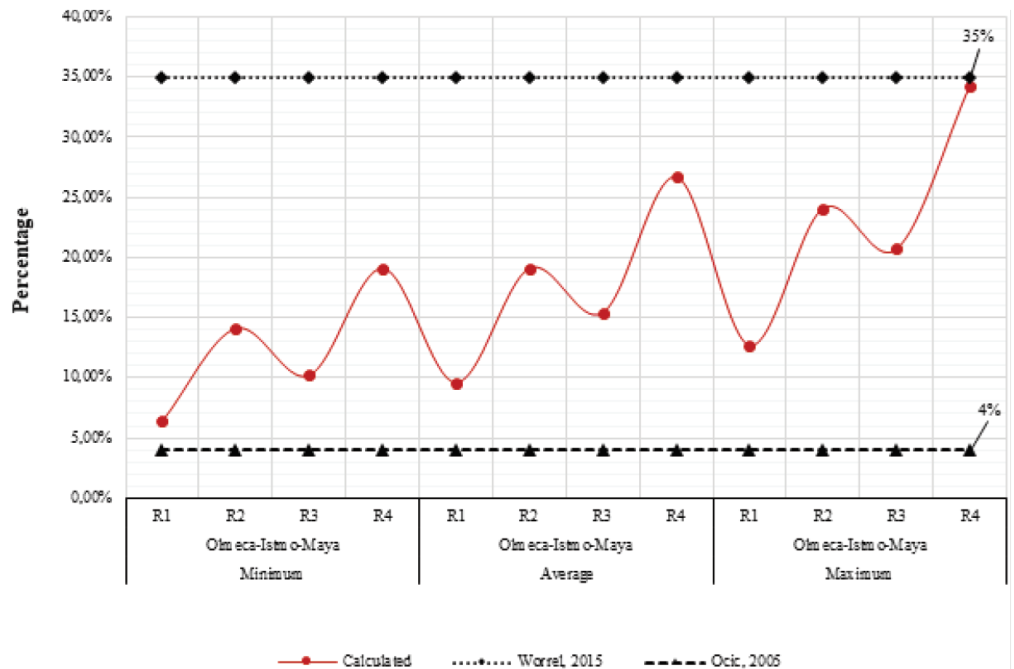
This figure shows that the calculated data for the equivalent energy consumption relative to the total processed crude is within the lower interval of the reference data cited by Szklo, 2005 (4 %), and within the highest reference as calculated with the data EPA, 2015 (35 %). Therefore, in analysis of the minimum energy consumption, the calculated interval lies between 6.4 % and 19.1 %, an average consumption between 9.6 % and 26.7 %, and a maximum consumption 12.7 % and 34.3 %. Additionally, an R4 refinery shows the highest equivalent energy consumption and an R1 refinery shows the lowest.
Conclusions
It may be thought that the quantity of required crude needed to satisfy the gasoline demand for the year 2030 is low (two million barrels per day), since it is equal to the quantity produced to date since the last couple of years. However, one has to consider that very complex refineries will be used which will be very efficient. On the other hand, when refining a lower quantity of crude, emissions, obviously, will be lower.
Refining very heavy oils in very complex refineries (R4) has a small disadvantage when considering energy consumption. Since the tendency in the very near future is precisely to extract this type of crudes in Mexico since these are the most abundant, then there will be no more solution than to bet for these types of refineries. This disadvantage may be compensated by their greater conversion efficiency and by using les quantity of crude to satisfy the demand and, consequently, will emit a lower quantity of atmospheric pollutants. Based on the scenario proposed by Bauer et al. (2003), that a strong economy increases the acquisition power of the population in order to obtain material goods (including automobiles), it also implies a greater quantity of atmospheric emissions. Therefore, an equilibrium should be reached between these two processes.
Among the consumed energy sources in the refineries to heat different processes, liquid gas may be the best option in terms of energy savings. On the other hand, its emission factors are low relative the other types of energy sources, except for natural gas (NG) which has lower factors for NOx and PM. The problem would then be evaluating which would be more convenient to obtain a greater socio-economic benefit: reduce emissions to the atmosphere or to lower operation costs of the refinery. The availability of an adequate energy source is also implicit, since sometimes the best option is not available or, it may be available at a higher cost. It all winds up in a cost-benefit study.
It is important to know the type of pollutant whose emission needs to be reduced if such were the case. If the problem is SOx, refinery gas (RG) would be the best option. If it were total particles (PM), one could either use fuel oil (FO) or refinery gas (RG).
Therefore, it is important to reach beyond the idea that “the best energy source is that one that pollutes the least”. Rather, one needs to analyze the advantages and disadvantages of using each one of them and their relation to the quantity of emissions to the atmosphere.
The use of electricity (EL) for the operation of pumps, compressors and ancillary equipment showed high emissions; this can be the consequence of its generation and distribution to the refinery, where some type of thermoelectric or carbo-electric source and not a different source of generation. The latter is because there is no information from PEMEX. However, if the pollutant quantity to used energy variables are analyzed, electrical energy shows a low relationship.
In relation to the different analyzed processes, the atmospheric distillation and vacuum distillation units should be emphasized since they are characterized by a high energy consumption. This means that their operation has serious implications relative to the product revenues and operation costs.
The complexity of a refinery in terms of a higher gasoline production yield is an important factor for energy consumption and atmospheric emissions.
Mexico’s possible refineries need to adapt themselves to different operation scenarios, such as changes in the crude’s yield, the quality of the product, variations in the prices of the crude and of the refined products.
It is important to develop and apply perspectives than maximize productivity and minimize energy consumption in constant change scenarios.
In relation with the energy reform in Mexico and the posture of the recently elected President (Andrés Manuel López Obrador), of building a new refinery, this document may help guide to the authorities of the energy sector to plan for a better yield in the production of gasoline and satisfy the possible demand for the future years, as well as minimize atmospheric emissions.
Finally, the demand for gasoline could vary in the future mainly due to the introduction of hybrid or electric vehicles, therefore it would be important to carry out research work that will consider this variable in the projection of the fuel.

