


 text new page (beta)
 English (pdf)
 Article in xml format
 Article references
 Send this article by e-mail
 Cited by SciELO
  Similars in
SciELO
Similars in
SciELO 
 Permalink
Introduction
Steam injection in mature oil wells is a dominant method used to improve the heavy oil recovery from the wells. Several studies have shown that for depths superior to 700 m is not an efficient method and it is not either economically rentable (Teknica Petroleum Services Ltd., 2001).
For the above reason, it is better to produce the steam deep inside the well. Among the problems that have to be solved in designing the steam generator (reactor) to be located at the well bottom, one of the most important is to provide an adequate cooling system to keep the wall temperature at an optimal level of security, especially on the combustion chamber walls. The available refrigerant, water in this case, must be allocated as a film on the wall to be protected. The benefits of the heat protection using a water film are still better when the film is perfectly adhered to the wall (when the wettability is good), when the film is stable (i.e. when there are few perturbations in the film-gas interface) and when the reduction of its thickness is small (when the interfacial atomization or evaporation rate is small).
Therefore, the problem of the thermal protection of the steam generator wall at the well bottom is located in the two-phase flow pattern nominated annular flow, and the point is basically to understand the hydrodynamic behavior of the liquid film when it flows concurrently with a core gas flow.
Annular flow
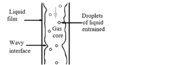
Annular flow is one of the most common flow patterns in two-phase flow. The annular flow is characterized by a core gas flow and a liquid film flowing on the pipe internal wall, with a wavy interface liquid-gas (Pravin et al., 2009).
At some relatively high gas velocities, the gas core drives part of the liquid as droplets. The liquid droplets entrained in the gas flow are formed by the atomization of the liquid wave crests due to the shear stress in the interface liquid-gas. Figure 1 shows a typical scheme of the annular flow pattern in downward film flow.
Interfacial waves
A typical characteristic of the annular flow is the presence of waves with several scales in the liquid-gas interface. In the technical literature regarding annular two-phase flow, it is possible to find information about different types of interfacial waves, but researchers agree that normally there are two types of waves present in this flow pattern, the so named surface waves and the perturbation waves (Zhu, 2004).
The surface waves have small amplitudes respect the liquid film thickness, their wavelength generally is measured in millimeters (Hewitt & Govan, 1990); their life time is short and most of the time they do not stand all around the pipe circumference. The perturbation waves which are also known as roll waves (Hanratty & Hershman, 1961), have a longer life time, and their amplitudes are generally several times the liquid film thickness (Asali & Hanratty, 1993).
For very low liquid velocities, the surface waves dominate the interface. Over a critical velocity of the liquid flow, the perturbation waves appear in the flow (Andreussi et al., 1985) and exert a strong influence on the film due to their dimensions and to their dynamic properties. Perturbation waves, as a difference from surface waves, exist in all the range of conditions producing annular flow.
In this study, waves are the result of the strain stress in the interface water-air, and that is why, they can be taken as a way of evaluating the film stability. If the crest is high and the wavelength is wide, two phenomena could take place: on one side, the film slims down in the valley and, on the other side, the probability that the crest atomizes is high; both mechanisms attempt against the film stability and against its average thickness.
Training phenomenon mechanism
In the annular flow technical literature, the term trained liquid, sometimes called atomization, has the same meaning of trained fraction (Coulson, 2003).
In this work, the trained liquid refers to the process in which is transported part of the liquid phase to the gas core as a result of the gas flow interaction with the liquid film, atomizing the crests of the waves and training them as droplets.
Generally, there are three mechanisms in which the liquid film is trained into the gas core in a downward vertical annular flow: a) training and atomization of the interfacial waves, b) training due to the explosion of the bubbles present in the liquid film, and c) training by the collisions between the droplets.
It has been widely accepted that after the perturbation waves, which are generated in the liquid film flow, the training wave is the liquid hauling mechanism which predominates, whereas the other two mechanisms have low impact.
Types of annular flow patterns
There are several types of downward annular flows, however, they can be classified mainly in three:
This type of annular flow consists of a liquid film with long waves having irregular amplitude, known as a non-stable system or torrent waves. The amplitude of these waves reduces with the increment of the gas volumetric fraction (Libreros, 2008).
The ideal annular flow, this type of annular flow pattern takes place when the gas volumetric fraction is very big compared to the hold-up, forming an ideal annular flow pattern. This schema has been widely used to obtain models of the velocity patterns and volumetric fractions of the liquid and the gas flows (Libreros, 2008).
The third type looks like the ideal annular model, where it is assumed that gas and the liquid flows are separated by a smooth interface. However, when the liquid flow is increased and at a certain critical gas velocity, the roll waves appear in the liquid film surface. This phenomenon has a periodical nature and travels over the liquid film at a velocity several times bigger than the average liquid film velocity. The roll waves front suddenly grows while its back part slims down gradually. The aspect of the roll waves coincides with its training which increases while the droplets are transported far away from the crest wave by the gas current. An additional increment in the gas flow will increase the presence of droplets in the gas core due to the atomization of the liquid film (that is the fog flow) (Levy, 1999).
The present investigation is focused on the experimental study of the downward vertical annular flow, to determine the liquid film thickness based on the pictures taken using a non-intrusive technique.
Experimental methodology
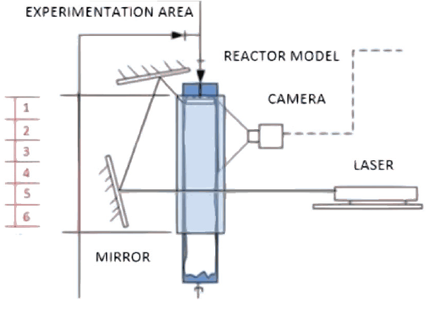
All experiments were undertaken keeping steady state conditions inside a vertical pipe. The set-up diagram is shown in Figure 2, it is formed basically for an acrylic pipe 1.300 mm long and 94.66 mm internal diameter with a 3 mm of thickness.
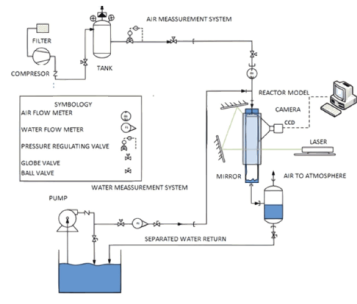
The first part of the work is focused on the description of the annular flow taking in consideration the both phases superficial velocities variation in order to generate such a flow pattern. The fluids used in the research are water and air which are easy to handle in a vertical pipe.
In order to generate the annular two-phase flow pattern in a downward vertical pipe, we took as a reference the diagram proposed by Swan & Afshin (2011), which is shown in Figure 3. In this diagram it is easy to determine the values of the superficial velocities of both phases (USG) and (USL) in order to reproduce the annular flow in the vertical pipe.
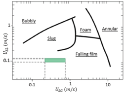
Figure. 3 Diagram proposed by Swan & Afshin (2011) for the downward vertical flow. The experimental zone is shown in green
The superficial velocities of each phase, are determined using the mass flow of the corresponding phase, the transversal area of the pipe and the density of the fluid, using the following equations:
According to the diagram proposed by Swan & Afshin (2011), the operation zone to obtain the annular two-phase flow is between the superficial velocities ranges of the phases shown below:
0.001 ≤ USG ≤ 10 [m/s]
0.001 ≤ USL ≤ 0.2 [m/s]
For our experimental rig in which we pretend to study the range of interest of air and water mass flows, the operation zone for these conditions is illustrated in the same Figure 3 and they are:
0.237 ≤ USG ≤ 0.773 [m/s]
0.099 ≤ USL ≤ 0.113 [m/s]
This is the set of conditions in which the steam generator will work in the bottom of the wells.
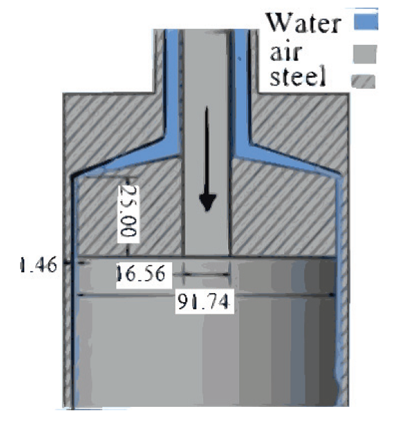
On the other hand, to generate the downward liquid film, a special geometry head, denominated inclined plate, was designed and manufactured. The inclined plate was to maintain the same area of liquid injection in order to have the same liquid velocity as far as the injection point into the internal part of the cylinder. The idea of maintaining constant the liquid transit area is to keep the same average velocity of the water along the plate, in order to supply the water in a gentle and uniform way. The advantage of the plate is, in principle, that the liquid injection does not induce perturbations of the film at the inlet to the vertical cylinder. It was monitored that the liquid velocity profile does not change abruptly before coming into the internal reactor wall, which will induce undesirable instabilities.
The base for the head geometry design is the average film thickness in millimeters computed using the Nusselt equation, to determine the thickness of a film slipping dawn on a vertical wall (Nusselt, 1916).
Where the Reynolds number Rew should be obtained (Wang et al., 2002), using equation:
On the other hand, according to the preliminary estimation of the combustion in the steam generator, the required water mass flow for cooling the reactor wall is 0.75 kg/s, and is the flow to be used in the experiments (Project SENER-CONACYT, 2016). So, the resulting Reynolds number is Re w = 10, 088 and the average film thickness determined with the Nusselt equation is δN = 1.46 mm.
This theoretical film thickness was used to specify the radial exit dimension of the liquid film from the head to the internal surface of the reactor. The head discharging the liquid into the cylinder has an annular shape as shown in Figure 4.
Three values of water mass flow were used for the experimentation, 0.70, 0.75 and 0.8 kg/s, and three values of air mass flow: 0, 1.86, 6.05 g/s. These values were determined with the operation conditions the reactor will have.
To obtain the film images a double pulsed laser Nd:YLF type, model LDY 303 HE mark Litron was used. The energy per pulse is 22.4 mJ with a wavelength of 527 nm (Green color). The laser is synchronized with a digital camera Speed Sense 9040 high resolution (1632 x 1200 pixels), with a 32 GB memory to get the images (Adrian, 2011; Prasad, 2000).
The camera is provided with a lens Nikon of focal distance of 24 mm-85 mm, in this research, a capture of 200 couples of images for each liquid mass flow studied was used, the conditions are shown in Table 1.
Table 1 Experimental matrix used in the research
| LIQUID |
LIQUID USL (m/s) |
GAS |
GAS USG (m/s) |
||
| Case A | 1 | 0.70 (42) | 0.099 | 0 | 0 |
| 2 | 0.75 (45) | 0.106 | 0 | 0 | |
| 3 | 0.80 (48) | 0.113 | 0 | 0 | |
| Case B | 1 | 0.70 (42) | 0.099 | 1.86 | 0.237 |
| 2 | 0.75 (45) | 0.106 | 1.86 | 0.237 | |
| 3 | 0.80 (48) | 0.113 | 1.86 | 0.237 | |
| Case C | 1 | 0.70 (45) | 0.099 | 6.05 | 0.773 |
| 2 | 0.75 (45) | 0.106 | 6.05 | 0.773 | |
| 3 | 0.80 (48) | 0.113 | 6.05 | 0.773 |
In Table 1, it is also possible to observe the sequence of execution of the experimental tests, it was decided to start without airflow, in order to take these results as a reference and then analyze the air flow effect on the liquid film behavior. Three runs were undertaken without air flow, just changing the water mass flow (Case A), three runs injecting one air flow for three liquid flow rates (Case B), and three runs with a higher gas flow rate than in case B changing the liquid flow rates three times, that is, nine runs at all. The run with a liquid flow rate of ṁL = 0.75 kg/s is analyzed the most, because is the condition to be used in the reactor with 100 % of thermal charge.
To execute a specific experimental run, once the experimental condition is fixed, a series of images is taken with the high-resolution camera lightening with the laser, all along the acrylic cylinder. Pictures were taken each 5 cm axially downwards, in a window of 5×3 cm2, i.e. in 6 observation zones, as shown in Figure 5. The images acquired were processed in order to determine the average film thickness in different axial positions.
Processing the information
For the film thickness measurement, an algorithm of MATLAB libraries for image recognition was used (The math works, 1994-2018). The algorithm of analysis, was able to use masked images which were imported from the software Dynamics Studio v3.20 (Dantec Dynamics, 2016).
The sequence followed for the image analysis algorithm is:
From the original picture (Figure 6a) the useless information is removed using a mask, and then with the resulting image, it is possible to determine the liquid film thickness along the 5 cm of the picture and the average liquid film thickness as well. It is important to remark that in this picture, the right edge coincides with the acrylic pipe internal wall which is the reference to measure the local thickness.
Figure 6b, shows the wavy film shape in the trimmed image, in all 200 images taken in the same position it is possible to measure the wave characteristics and the axial film thickness variation. The algorithm helps to determine the liquid film thickness through the image analysis, in all the different experimental conditions. The radial variation of the gray gradient is determinant to differentiate the liquid film zone, for instance, in Figure 6b it is possible to observe that the edge of the film is found when the black radial gradient indicates an inflection point
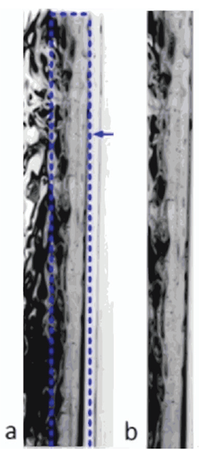
Figure 6 a) Original image showing the areas to be removed, b) image trimmed using a mask to remove useless information
This procedure is repeated in a determined number of points axially in the picture, following the flow direction, and then connecting all of them, the shape of the interfacial wave of the liquid film was obtained, and in a determined axial point also the local film thickness (Adrian, 2011).
First of all, the image is charged from a file located in the memory of the PC having the images to be analyzed. All pictures must be in a JPEG format, in a gray scale of 8 bits (in a value of pixel from 0 to 255), this is the format in which the Dynamics Studio v3.20 software allows to export the image and MATLAB supports it.
The set of exported images are called from the algorithm “film thickness detection” and works as follows:
A certain number of images are read by the code, and its wide and height are dimensioned. The limits are defined enclosing the relation between the intrinsic coordinates anchored to the files and columns of each dimensional image and the space location of the same file and column in a common coordinate system. For each image, its coordinate system is unique, that is, in two images there are two distinct coordinate systems and they cannot interact in between, for this reason, it is necessary to have a universal coordinate system or common which permits that each image interact with the others. This system is called World Coordinate System (McKenna & McGillis, 2002). The image is shown regularly in the planar system World-X and World-Y so that the intrinsic values X are aligned with the world values X, and the intrinsic values Y are aligned with the world values Y. The pixel space from file to file does not need to be equal from one column to the other. The intrinsic coordinates are defined in a continual plane while the sub index locations are discreet with integral values. Fixing one value of scale (mm/pixel) which are multiplied by the world limits in X and Y, the given image is ordered according to a specified by the scale (The math works, 1994-2018). In order to produce an interaction or information flow in computer graphs, it is necessary that the coordinate system of each model or image be transformed to the world coordinate system, and then the morphologic analysis could be executed.
Conversion images to binary images based in a threshold, is a simple, and effective, way of partitioning an image into a foreground and background. This image analysis technique is a type of image segmentation which isolates objects by converting grayscale images into binary images. Image thresholding is most effective in images with high levels of contrast. The resulting images replace the binary inlet images with amplified luminance assigning a value 1 (white) and replace the pixels with minimal illumination with a value 0 (black). With the above mentioned action, the level of illumination is specified in a range ;, this range is relative to the level of grey in the image. Then, a 0.5 value is half way between white and black, independent of the each image scale (González & Wintz, 1987).
Pixel smoothing and contour recognition. Here the external limits or contours are outlined. The pixel smoothing consists in a local average of the values of each pixel and its neighbors (we took four neighbors for each pixel) so that in the resulting images, brightness and reflex are rejected.
Identification of the contour of the pipe. In the step three, the function used from the MATLAB library outlines the objects when they are son or father, that is, it encloses the identified object.
Identification of the contour of the interface liquid-gas. The contour identification consists in determining the set of points corresponding to the interface, each point is joined to its neighbor, giving as a result a set of picks which later on, will be adjusted with a Gaussian type model.
Film thickness. The numerical data of the liquid interface is a file vector, so when the numerical data of the pipe contour are subtracted, its transposed provides the film thickness as a result.
The coordinates position which outline the pipe is the minimal horizontal coordinate among all the identified contours (zero position to start the film thickness calculations). The contour with more points in the coordinates is the interface contour, which is a closed contour and is a sub set of points accomplishing the conditions of distance to the edges or distance between neighbor points which allows to recognize the interface liquid-gas.
Once identified the contour in each axial position, the image could be printed, showing the axial shape of the interface liquid-gas, so the axial variation of the liquid film thickness, type of wave, length of wave and average velocity are determined.
Results
A visual evaluation was done to all the pictures taken, from which the observations of the downward film behavior, with and without interaction with a concurrent gas flow, are provided.
The following figures show the film behavior without interaction with a core gas flow i.e. the gas flow in this case is zero (Case A)
Figure 7 shows the axial film thickness for three different Reynolds numbers along the first 5 cm, from the injection point. According to this behavior, the following comments can be made:
With the biggest tested Reynolds number Re w = 10,360 (Figure 7c), the interface gas-liquid is more wavy and the film seems to be thicker for this flow rate.
The waves are so mixed, that a single wave mixed with others is difficult to separate (an individual wave has a big amplitude and velocity).
Some little bubbles start appearing in the liquid film when its flow is increased, i.e. when the liquid trains air into the liquid film.
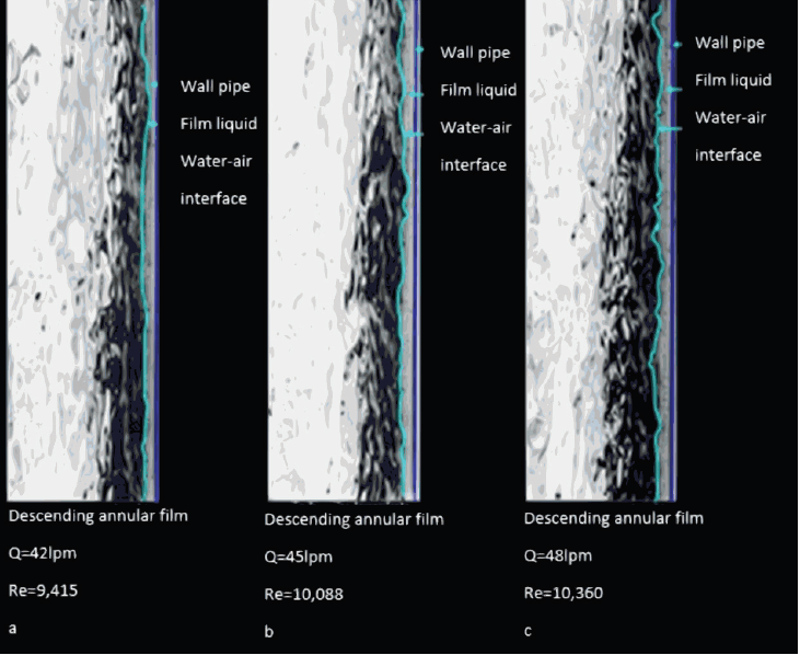
Figure 7. Downward annular film, without any flow of air, case A, along the first 5 cm from the inlet
Figures 8 and 9 show the downward liquid film flow behavior when it interacts with a concurrent air flow (cases B and C).
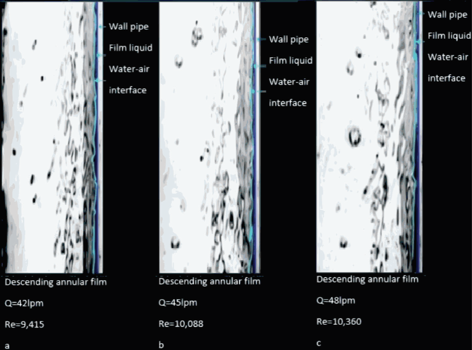
Figure 8 Downward annular film, with a concurrent air flow, ṁG = 1.86 (g/s), case B, along the first 0.05 m from the inlet
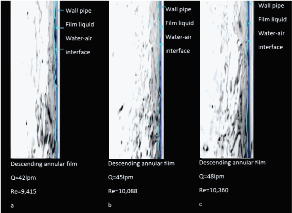
Figure 9 Downward annular film, with a concurrent air flow, ṁG = 6.05 (g/s), case C, along the first 0.05 m
According to the Figure 8, there is an effect of interaction between the liquid film and the air flow, which can be resumed in the following:
The interaction of the air flow and the liquid film produces a ripples reduction in the interface.
Regarding the training mechanisms, the only one appreciable by means of the photograph technique was the wave training.
Probably the interface liquid training comes along with the crest atomization, reducing the film mass flow and its thickness.
When the air flow is increased as far as 6.05 g/s (Figure 9), the film behavior along the first 5 cm from the inlet is as follows:
There are no perturbation waves due to the interaction of the air flow with the liquid film.
The liquid film seems to be thinner than in the other cases studied, and it moves faster because it is trained by the air stream.
The air flow does not permit the local film to increase its thickness on the wall, provoking that the crests flatten, avoiding its formation. Here the atomization of the crest is more probable, so it contributes that the film lose mass and consequently thickness.
Film thickness, without air flow, case A
The captured images were processed using the algorithm before mentioned. Around 40,000 film thickness measurements were obtained for each liquid mass flow in different axial zones of observation, that is from z = 0.05 to 0.30 m. The average values of the film thickness, temporally and spatially, in each zone of observation, for each one of the liquid mass flow are presented in Figure 10.
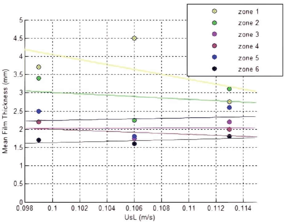
Figure 10 Average of the film thickness, without gas flow, case A U SG = 0 m/s along the length z = 0 to 0.3 m
For the liquid injection head design, it was considered a vertical annular section producing a film of the same opening thickness moving down on the vertical wall, only for the action of the gravity force, this case is taken as a reference flow. As mentioned before, the separation between the plate and the acrylic pipe internal wall is equal to the film thickness provided by the Nusselt equation for the reference flow. However, in the same channel, a smaller and a bigger flow than the one taken for the design were introduced. In principle, when a small flow is introduced in the same opening, it is oversized and when the flow is bigger than the one of reference, the channel is undersized for this flow, that is, the geometry of the head has an important influence on the induced behavior of the liquid film.
The average thickness was obtained of 400 pictures taken in each axial observation zone (position in zi, ti) and taking into consideration that in each instant there is a different average film. Therefore, it is necessary to obtain a local and temporal average of the film magnitude, so that by allocating all this averages in an axial way we obtain the average profile of the film thickness.
The temporal average thickness at an axial position zi in each observation zone is determined by means of the equation
With this, we obtain a time averaged picture in the first 5 cm, that is, from z = 0 to z = 5 cm, and then it is possible to determine, the local average film thickness in the first observation zone z = 0 cm to z = 5 cm,
In equations (6) and (7), t_i represents the time in which each of the 400 images were taken and n is the number of axial points taken in each observation zone (axial image length), where the local and temporal average film thickness was computed
By repeating this procedure to each one of the six observation zones along x, it can be observed the axial variation of the film thickness and then its stability.
According to Figure 10, there is an entry influence and the action of the gravity tends to accelerate the film, so that the film thickness decreases axially.
While the film goes down, its thickness is reduced because its average velocity is increased by the gravity acceleration, in all flow cases this behavior seems to be the rule. In the zones 1 and 2 it can be observed more oscillations due to the entry and after the zone 3, the oscillations are more stable.
Film thickness, with air flow, cases B and C
For cases B and C, the average thickness was obtained using the same procedure than in case A (Figures 11 and 12).
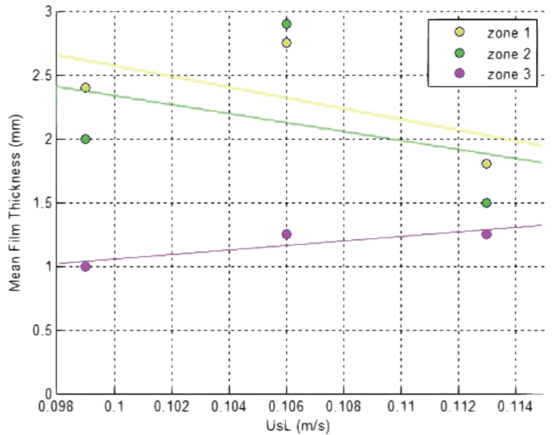
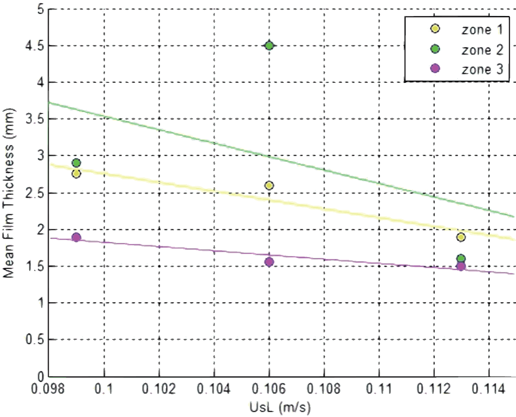
Figure. 12 Average film thickness, case C, USG = 0.733 m/s along the axial length of z = 0 to z = 0.15 m
According to the obtained results in each tested flow (Figures 11 and 12), it is possible to observe that when the film goes down it tends to reduce its thickness. In some cases, data was taken only in three observation points because we considered more important the 15 first centimeters. In this region it is possible to observe the effect of the head discharge of the film into the cylinder and how it develops descending the wall.
The superficial gas velocity (U SG ), has a big influence on the liquid flow because the film thickness for a same liquid flow rate reduces when the air flow is increased, which means that the shear stress of the interface liquid-gas drags the film to the bottom and the liquid film moves faster. The action of the gas phase over the liquid film, has as a consequence, changes in the value of its thickness, it also affects the distribution of the downward film, and the shape of the interface.
The liquid film is susceptible of perturbations due to the gas flow, which provokes its slimming in the flow direction, which is due to the strain stress in the interface liquid-gas. However, in the first 10 centimeters there is an air vortex due to the air jet impingement on the pipe wall which provokes that the film thickness increases initially in the entry and then diminish. When the liquid flow is increased the effect is less notorious.
For all above, handle the gas velocity in a convenient range will help to improve the uniformity of the liquid film, however, if the gas velocity is too big, it could happen that the liquid film has ruptures, and then the wall has the risk to dry, increasing the droplets flow, as shown in Table 2
Table 2 Average film thickness along the first axial 15 cm in the steam generator
| USL (m/s) | USG (m/s) |
|
|
|
|---|---|---|---|---|
| 0.099 | 0 | 3.7 | 3.4 | 3.9 |
| 0.106 | 0 | 4.5 | 2.25 | 1.75 |
| 0.113 | 0 | 2.75 | 3.1 | 2.2 |
| 0.099 | 0.237 | 2.4 | 2 | 1 |
| 0.106 | 0.237 | 2.75 | 2.9 | 1.25 |
| 0.113 | 0.237 | 1.8 | 1.5 | 1.25 |
| 0.099 | 0.733 | 2.75 | 2.9 | 0.9 |
| 0.106 | 0.733 | 2.6 | 4.5 | 1.6 |
| 0.113 | 0.733 | 1.9 | 1.5 | 1.5 |
Unlike the other existing techniques, local (capacitive, conductive and radioactive probes) and spot metering (needle probe, hot wire, optical fiber and laser dispersion), the technique proposed in this work is of the spatial type, which shows the film thickness in several points simultaneously, in different sections of the liquid film, in order to extract the most precise structure. Additionally, the proposed technique is nonintrusive as are not most of the spot metering ones, and it has not a limited height of study as the local techniques.
Conclusions
An experimental study of a vertical downward annular flow to determine the thickness and stability of a falling film water flow was carried out. A special annular header for the liquid injection was designed and built, its dimensions are to handle the liquid flow required by the reactor design, when it works at 100 % of its capacity. The annular shape of the water injection head was dimensioned to maintain uniform the injection area, radially and axially as well. This design has the purpose to reduce instabilities produced by the variation of area and velocity, and then we attend to have a smooth entry and exit of the cooling liquid. The experimental information here presented corresponds to a straight vertical film.
Some experiments were undertaken without air flow in order to take the results as a reference. In this set of experiments, we observed that any increment of the liquid mass flow produces a thicker film, but the interface waves also grows. Initially the pipe is full of air at atmospheric pressure, so to maintain the non-slip condition in the interface, the air is dragged by the liquid film forming a vortex in the gas phase, which has an important role in the film behavior. In regard to the film velocity, it increases axially due to the gravity effect, so the thickness decreases proportionally to guaranty the mass conservation.
In the other set of experiments, with gas flow, in principle when the gas flow is increased, the film thickness decreases. This behavior shows that there is an effect of the strain stress in the interface and probably exists an atomization of the liquid film in this zone at some critical gas velocity. An important point to keep in mind is that the gas injection was done only using a central nozzle, so that the cone formed by the gas jet has an impact point on the wall and of course there the film thickness is thinner and a gas vortex is also formed going upward and it is one of the factors that makes thicker the film in the inlet zone.
The experimental technique used, quick photograph and image recognition showed to be useful to determine the average film thickness which always was between 1 and 4.5 mm. It was also observed that the smooth film presents such characteristics that allow it to protect thermally the reactor internal wall, because it presents low waviness in the interface, and in principle its rupture and atomization is less probable.
When the air flow is increased, the drag in the interface liquid film-air also increases and probably there is atomization, which is the reason why the film slims.
The results here presented have certain limitations because only is taken the axial variation of the film thickness in one angular position of the acrylic pipe, however, statistically provides an idea of what happens in all the internal wall of the cylinder.
To complete the analysis, it would be necessary to determine the radial and axial variation of the film average velocity, which is part of a future work, similarly to the injection effect of four symmetrical jets of air and one central
Finally, the technique used in this work has proved to be useful for the analysis and comprehension of a vertical downward annular film concurrent with a jet of gas.
Nomenclature
AG |
Area section occupied by the gas - m2 |
AL |
Area section occupied by the liquid - m2 |
AT |
Total area of the pipe - m2 |
DT |
Internal diameter of the pipe - m |
g |
Gravity acceleration - m/s2 |
n |
Number of points considered |
ṁG |
Gas mass flow - g/s |
ṁL |
Liquid mass flow - kg/s |
P |
Pressure - Pa |
Rew |
Reynolds number proposed by Wang |
ti |
Instant in which the image was taken - s |
T |
Period in which the whole 400 images were taken - s |
USG |
Gas superficial velocity - m/s |
USL |
Liquid superficial velocity - m/s |
Uf |
Film velocity - m/s |
z |
Medium axial position in each observation zone - cm |
zi |
Actual axial position in each observation zone - cm |

