


 text new page (beta)
 English (pdf)
 Article in xml format
 Article references
 Send this article by e-mail
 Cited by SciELO
  Similars in
SciELO
Similars in
SciELO 
 Permalink
Introduction
The Finite Element Method (FEM) in order to analyze cancellous bone is commonly used for simulations of mechanical tests on models that represent its structure.
A method for creating these models uses data from high resolution microtomography, which directly perform a tridimensional model of the structure through scanning.
However, this method specifically depends on the micro CT resolution. Bevill and Keaveny in 2009 made models, using this method, to be analyzed later by FEM varying the voxel size.
In other cases, it has been preferred to modify the cubic form of the voxels to generate better results, like Depalle who in 2013 changed that shape to a hexahedral and similarly modified the voxel size to get closer results to reality (Depalle et al., 2012).
Other models are based on the trabecular bone representation by a repetition of unit cells to create a complete structure. Kowalczyk (2003) generated various models using this kind of representation.

Figure 1 Variation of a trabecular bone model of femoral neck at different voxel sizes: a) 20 μm and b) 120 μm (Bevill and Keaveny, 2009)
In other cases, it was chosen to make two-dimensional models to generate a representation of an image that shows a trabecular bone structure. Ramírez et al. (2010) generated two-dimensional models from cancellous bone images obtained by optical microscope, using representations from Voronoi cells.
Other kind of representation idealized each trabecula of a structure using geometric figures. Saha and Wehrli used a methodology based on this in 2004, where they used ellipses to represent each trabecula by scanning points on their periphery, and also a color code was used (Saha and Wehrli, 2004).

Figure 2 Variation of a vertebral trabecular bone model, with hexahedral voxels of different sizes: a) 20 μm and b) 80 μm (Depalle et al., 2012)

Figure 3 a) Example of unit cell to represent cancellous bone b) Structure generated by a unit cell (Kowalczyk, 2003)

Figure 4 Two-dimensional cancellous bone model through Voronoi cell technique: a) representation and b) representation of equivalent von Mises stress for a compression test (Ramírez et al., 2010)

Figure 5 a) Ellipse as representation of a trabecula generated by a scanning method, b) color code for an image of trabecular bone to assign trabeculae dimensions and orientations (Saha and Wehrli, 2004)
Methodology
The methodology is based on Saha and Wehrli paper, because a similar representation is used for each trabecula of a structure. The images to develop this methodology were obtained from a bovine femoral specimen, because it is easier to get the samples than from human bone specimen. Subsequently, a portion of the upper epiphysis was selected. That portion was immersed in boiling water, to remove fleshy tissue and red marrow, this process took about 3 hours, under constant water changes. The next step was to immerse the specimen in a hydrogen peroxide solution to 3.5%, in order to detach the remaining residues after boiling. This process took about 16 hours. Once the previous steps were done, it was possible to observe in a better way the trabecular structure, which permitted to identify three significantly different regions:
Region 1: the trabeculae do not have a preferential orientation. It was seen from greater trochanter to the area named as Ward's triangle.
Region 2: the trabeculae are oriented diagonally to the direction of the femoral head. This region was seen in the femoral neck and in a previous area to the femoral head.
Region 3: the trabeculae do not present preferent orientation, however their thickness is visibly greater than the trabeculae in the previous regions. It was seen in the area of the femoral head.
Rectangular areas (2 cm long, 1 cm wide) were selected on the trabecular surface of the specimen (Figure 6).

Figure 6 Femur section after removing remaining tissues and analysis areas: region 1 (blue), region 2 (green) and region 3 (red)
The reason for selecting areas of that size is to represent the area of the intermediate parallel plane to the main axis of a cylindrical trabecular bone specimen for a compression test. The Figure 7 shows the images of three regions marked by ink.

Figure 7 Trabecular bone images, where the different regions of the specimen are showed: a) region 1 b) region 2 and c) region 3
Then, first coordinates were taken assigning middle points in each trabecula of the cancellous bone, being complex geometries the assigning was performed by the operator. Figure 8 shows an example of midpoints assigned to each trabecula.

Figure 8 Midpoints assignation for some trabeculae in cancellous bone. Image at 200X (Narváez, 2004)
In the methodology of Saha and Wehril (2004) a method of scanning was used on the trabeculae to generate the respective ellipses, in this case, that scanning was omitted and instead two points were directly taken from the trabecular bone image.
One of the points is taken at the trabecula union zone. This point aim is to obtain major axis of the ellipse, based on the calculation of the distance between this point and the midpoint. The second point was taken at the edge of the corresponding trabecula, this point should be at an angle of 90 degrees to the trabecula major axis, which allowed calculating the ellipse minor axis.
The inclination angle of the ellipse was calculated generating a vector between the center point of the trabecula and the point obtained to calculate the major axis, the angle of this vector was obtained and this was considered as the inclination angle. Figure 9 shows the points and the inclination angle for one trabecula.

Figure 9 Process to represent trabeculae from ellipses: a) points assignation to calculate the major axis (blue) and the minor axis (green), from the central point (red) and b) inclination angle of the ellipse
From the above points it may be generated a representation with ellipses of a whole trabecular structure, this representation was useful because the later construction of the model in Abaqus™ through Python™ programming language, needed an assignation of a number to each ellipse in order to build two lists.
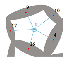
The first list was named pores list, it is associated with the pores within the trabecular structure. This list contains other lists, which indicate the ellipses that are around every pore. That means the internal lists amount equals the pores amount. The second list was named contour list, it is associated with ellipses that are on the periphery of the obtained structure, in order to get an outline to the final model. The amount of elements of the second list should be equal to ellipses amount that are on the periphery of the representation. Figure 10 shows the described previous steps, using an example of a trabecular structure represented by ellipses.

Figure 10 Previous analyses that were required to build the model: a) assigned numbers to each ellipse, b) ellipses that surround a pore (orange) and c) contour ellipses that help to form the outline of the model (green)
The models construction process was done to generate a programming code to take data from the points coordinates obtained from the trabecular bone image, the pores list and contour list. In order to obtain the corresponding points to each pores, first it was programmed command lines that calculated an intermediate point on each pore, and then a vector was generated from central point of each trabecula to central point of corresponding pore (pore vector). This was controlled by the pores list. Figure 11 shows a midpoint of a pore and the respective pore vectors to each corresponding trabecula.
Then, a function was defined to make a comparison between angle of pore vector and the inclination angle of each ellipse. If the inclination angle were greater than the pore vector angle, the angle value of pore vector would be subtracted to the inclination angle, if the subtraction were less than 180° a tangent point on the corresponding ellipse would be placed at an angle 90° less than the inclination angle of the ellipse, if it were greater, the tangent point would be placed at an angle 90° higher. If the inclination angle were less than the pore vector angle, then the value of inclination angle would be subtracted to the angle value of pore vector, if the subtraction were less than 180° a tangent point on the corresponding ellipse would be placed at an angle 90° higher than the inclination angle of the ellipse, if it were greater, the tangent point would be placed at an angle 90° less.
For generating the curve which delimits the contour of the model using the spline tool, it had to be defined within the programming code some instructions to obtain tangent points to the ellipses.
Figure 12a shows the sketch made by spline tool that represents pores and outline of the used example. Figure 12b shows the two-dimensional model generated by Abaqus™.

Figure 12 Two-dimensional model for an example of trabecular bone: a) sketch made by the spline tool and b) two-dimensional model built from the described methodology
After the models were generated, they were cut through Abaqus™ tools to contain each model in a rectangular area (2 cm x 1 cm).
That was done to represent the area of the intermediate parallel plane to the main axis of a cylindrical trabecular bone specimen (Figure 13).

Figure 13 The cut of each model to delimit them in a rectangular area: a) frame in Abaqus® that made the cut and b) model that has been cut
The models that were generated using this methodology from the selected regions, are shown in Figure 14. In turn, Table 1 shows the most relevant data about each model.

Figure 14 Trabecular bone models generated by the described methodology for the different regions: a) region 1, b) region 2 and c) region 3
Table 1 Relevant data about generated models
| Model | Amount of trabeculae | Amount of pores | Trabecular average thickness [mm] | Trabecular preferential orientation | Area fraction |
|---|---|---|---|---|---|
| Region 1 | 532 | 196 | 0.258±0.073 | 80°-105° | 48.39% |
| Region 2 | 619 | 209 | 0.257±0.077 | 55°-80° | 54.39% |
| Region 3 | 1120 | 375 | 0.251±0.058 | 75°-100° | 65.6% |
In order to test the models, a simulation of a mechanical compression test was conducted using Abaqus™, very simple conditions were assigned, because it was only intended to show that the methodology is useful for generating closer models to reality. First, a restricted movement condition was established on the base to each model, also a self-contact condition without friction was assigned to the trabeculae of each model and in each one was used a triangular elements mesh. Moreover, plane stress conditions were considered for each simulation. Then an analytical rigid part was placed on the top of each model, which moved 0.89 mm, this value corresponds to 5.5% deformation (Ramírez et al., 2010). Among each model and the compression plate it was assigned a friction coefficient equals 0.27 (Davim and Marques, 2004).
In turn, the material properties were considered isotropic. A Young's modulus of 1.678 GPa was assigned, that was obtained using empirical formula of Rho (1993) from a bulk density equals 0.4 g/ cm3 (Guerrero, 2014). Furthermore, it was established a Poisson's ratio equals 0.3 and it was assigned a density equals 1.8 g/cm3 (Ruiz, 2010). Also, it was considered a maximum compressive strength equals 100 MPa (Cowin, 2001).
Results
This section shows the results about the compression tests. The first model used a mesh with 23,950 triangular elements.
Figure 15a shows the stress level in this model through a color scale, where the gray areas are those that have exceeded the maximum strength. In this analysis, it can be seen that only some trabeculae in this structure have exceeded the maximum strength, they are mainly in the section near the base, in the upper right corner area and some intermediate trabeculae. That means the load distribution along the structure focuses on these described sections.

Figure 15 Von Mises stress level for three generated models at 5.5% strain: a) region 1, b) region 2 and c) region 3
The second model used a mesh with 30,692 triangular elements. Figure 15b shows the stress level through the structure. Areas that have overcome the strength value include some diagonal trabeculae localized from the lower left corner to the upper right corner of the model, then, the trabeculae that have failed are those that have a preferential orientation and load is transmitted through this zone.
For third model that corresponds to region 3, the used mesh contained 40,245 triangular elements. Figure 15c shows the stress level through structure. If it is compared with previous models, this model has a greater number of zones with a different color to blue, that means, the most elements in this structure are working to distribute the load, so then it is performed a uniform stress distribution.
Figure 16a shows a comparison about the reaction force versus displacement curves of three models.

Figure 16 a) Reaction force versus displacement of each model and b) maximum reaction force versus area fraction of each model
This graph shows the apparent slope changes in model 2 compared to the other two models, this happened because interactions occurred among the trabeculae.
It can be appreciated that third model presents the strongest reaction force of three models, this is because it is the model that has the largest area fraction and also it has an adequate architecture for the established load.
Furthermore, figure 16b shows a graph about maximum reaction force versus area fraction for the three models, in this graph it can be seen, how the area occupied by a model causes variations in the reaction force.
It is important to say that the area fraction can be considered equal to the volume fraction (Ruiz, 2013). However, it should be noted that the reaction force does not increase linearly with the area fraction, this is due to the architecture of each model.
When comparing these three models using percentages, it can be seen that the model 2 has a 12.6% higher area fraction than model 1, and in turn it has a 23.8% higher reaction force than model 1. Model 3 has a 20.61% higher area fraction and a 73.54% higher reaction force than model 2. Furthermore, model 3 has a 35.81% higher area fraction and a 114.86% higher reaction force than model 1.
Conclusions
For proposed methodology, in terms of models that can be obtained, the final geometries and structures that can be represented are very similar to the geometries and structures that appear in the original images. This is corroborated by three obtained models in this work, because each one represents a different trabecular bone image.
At the simulations, it was possible to see that the different architectures and different area fractions, affect the final results, both the failure regions and the behavior of the graphs about reaction force versus displacement and maximum reaction force. Furthermore, the shown percentages confirm the area fraction effect in the structure stiffness, where model 3 had considerable percentage increases, because it had 20.61% more area fraction than model 2, this increased its reaction force 73.54% more, however this is most clearly seen when comparing model 3 and model 1, where model 3 had 35.81% more area than model 1, this caused that reaction force increased by 114.86%, that is, it was more than double what model 1 could give.
Because in each simulation the same characteristic test parameters and the same mechanical properties were established, the difference among results depends only on the structure formed by the trabeculae and area fraction occupied by bone.

