


Services on Demand
Journal
Article
 English (pdf)
 Article in xml format
 Article references
 Send this article by e-mail
Indicators
-
 Cited by SciELO
 -
 Access statistics
Related links
-
 Similars in
SciELO
Similars in
SciELO
Share

 Permalink
Ingeniería, investigación y tecnología
On-line version ISSN 2594-0732Print version ISSN 1405-7743
Ing. invest. y tecnol. vol.16 n.4 Ciudad de México Oct./Dec. 2015
An Approximation to the Probability Normal Distribution and its Inverse
Una aproximación a la distribución de probabilidad normal y su inversa
Alamilla-López Jorge Luis
Instituto Mexicano del Petróleo, Dirección de Investigación en Transformación de Hidrocarburos. E-mail: jalamill@imp.mx
Received: February 2015.
Accepted: March 2015.
Abstract
Mathematical functions are used to compute Normal probabilities, which absolute errors are small; however their large relative errors make them unsuitable to compute structural failure probabilities or to compute the menace curves of natural hazards. In this work new mathematical functions are proposed to compute Normal probabilities and their inverses in an easy and accurate way. These functions are valid over a wide range of random variable and are useful in applications where computational speed and efficiency are required. In addition, these functions have the advantage that the numerical correspondence between the random value X = x and its Normal probability Φ (-x) is bijective.
Keywords: normal distribution, inverse, absolute error, relative error.
Resumen
Se utilizan funciones matemáticas para calcular probabilidades normales, cuyos errores absolutos son pequeños; sin embargo, sus grandes errores relativos las hacen inadecuadas para calcular probabilidades de falla de estructuras o para calcular curvas de amenaza de peligros naturales. En este trabajo se proponen nuevas funciones matemáticas para calcular probabilidades normales y sus inversas, de manera fácil y precisa. Estas funciones son válidas en un intervalo amplio de valores que puede tomar la variable aleatoria y son útiles en aplicaciones donde se requiere velocidad y eficiencia computacional. Además, estas funciones tienen la ventaja de que la correspondencia numérica entre el valor aleatorio X = x y su probabilidad Normal Φ (-x) es biyectiva.
Descriptores: distribución normal, inversa, error absoluto, error relativo.
Introduction
The normal distribution function Φ (-x) is used in engineering probabilistic applications to compute reliabilities of structural systems such as buildings, offshore platforms, pipelines, tanks, and bridges, among others. These applications require accurate estimations of small probabilities, which are associated with relatively large values. In addition, these probabilities have to be easily invertible. The disadvantage of not having a closed analytical form of estimation Φ (-x) has been overcome using mathematical approximations. Summaries of these mathematical approximations are given in (Abramowitz & Stegun, 1972; Patel & Read, 1996), which are useful to compute probabilities or their inverses, but not both. The errors of these approximations are specified in terms of their maximum absolute error. The absolute errors of the approximations are small but their relative errors are significant, which becomes important in the tail of probability distribution. In the present work, this inconvenience is shown for the best mathematical function reported in (Abramowitz & Stegun, 1972), the one with minimum absolute error among the available approximations. Also, other approximations commonly used to compute failure probabilities are revised and new mathematical expressions with no such inconvenience are proposed. These new functions are useful to compute Normal probabilities and their inverses in a relatively easy and fast way, with good accuracy. Furthermore, they have the advantages of being valid over a wide range of the random variable, which makes them useful in engineering applications.
Reference framework
Herein, some of the mathematical functions typically used in engineering applications are reviewed. The number of functions analyzed is not exhaustive; the author only discusses some approaches that in his opinion are representative for estimating probabilities and/or their inverses in structural and mechanical engineering. The analysis is focused on identifying the accuracy and scope of these functions, and showing the inconveniences mentioned in the previous section.
In general, the normal probability distribution function Φ (·) can be described in terms of its probability density function φ (·) as follows.

The function ψ(·) relates the normal distribution function with its derivative, the probability density function φ (x). It can also be seen as the one that transforms the probability density function in its cumulative. Herein, to obtain values of ψ(·) for large values of x, the first and second derivatives ψ(·) are taken: ψ', ψ'' respectively, hence it gives the linear second order differential equation.

This differential equation was solved numerically for the initial conditions ψ (x = 0) = and ψ' (x = 0) = –1. Such a solution is taken as reference for ψ (·) . As shown in Figure 1, the asymptotic approximation to describe ψ (x), given by the expression (3), gives good results for large x values.


For x values close to zero, Eq. (3) , diverges from the corresponding numerical function. Although the asymptotic approximation of this function can be used to calculate probabilities associated with large values of x , it has the disadvantage of not being easily invertible.
Two functions to describe ψ (x), that provide good approximation over a wide range of x values, are those proposed by Hastings (Abramowitz and Stegun, 1972; (Rosenblueth, 1985). The Hastings's approach is a classic function, probably the most used to compute Normal probabilities, because it has the minimum absolute error in ( Abramowitz and Stegun, 1972), and can be expressed as follows.

where aj are coefficients with ten significant figures, j = 0, 1, ..., 5. This approximation gives absolute errors εA, lower than |εA (x) < 7.5 × 10⁻⁸|. However, as is shown in Figure 2, the relative errors εR grow significantly with x. This can also be seen in Figure 4 , where the corresponding function ψH (·) diverge from the function obtained numerically as x grows, which means that the accuracy of the approach should be expressed in terms of its relative errors, not by its absolute error. Likewise, an inconvenience is that Eq. (4) cannot be easily inverted.

The function proposed by (Rosenblueth, 1985) to describe ψ(x), can be expressed as
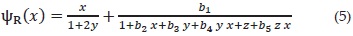
Where bi , i = 1, ..., 5, are numerical coefficients, y = x2/2, and z = 2.93 y2. As is shown in Figure 3, and according to the author, this last function leads to relative errors below |εR (x) < 4.5 × 10⁻⁵| when x>1 and relative errors are below |εR (x) < 2.0 × 10⁻⁴| over a wide interval. As it is shown in Figure 4, this approach is better than that by Hastings, because match up very closely with the numerical ones solution. However Eq. (5) can only be inverted numerically.

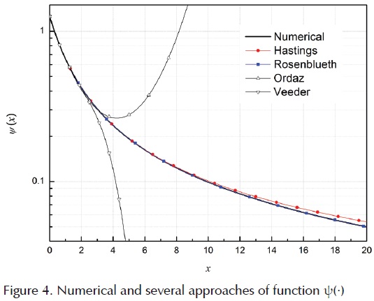
There are other expressions, as that proposed by Veeder (1993) and Ordaz (1991) , which have the advantage that the estimation of probabilities and their inverses are easy. However, the relative error grows a lot for x values greater than (3). In Figure 4 , the function ψ(·) associated with these last approaches is compared with that obtained numerically and in general, the accuracy of these approaches should be expressed in terms of their relative errors; not by their absolute error, because this leads to compare errors associated with probabilities of several magnitude orders.
Normal probabilities
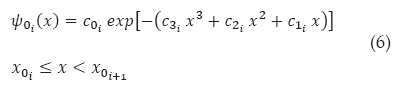
In this work, the mathematical expressions to describe the Normal distribution are specified in terms of its complement, which indicates that for x >> 0 values, Φ (-x) → 0. However, it is possible to compute Normal probabilities greater than 1/2, because of the symmetry of this function, Φ (x) = 1 - Φ (-x). Herein, ψ (·) is described by a set of three functions ψ0i (·), i = {1, 2, 3}, which have the same mathematical form and are given by Eq. (6) . Each one of these functions are valid for the interval [x0i, x0i+1], i = {1, 2, 3}, where x0i and x0i+1 values define the boundary of contiguous intervals, specified in Table 1.
Parameters and coefficients values of the proposed approach.
The function ψ(·) decreases as a function of x. The exponential function given by Eq. (6) is suitable for describing that decrement, because its behavior is decreasing. The third degree polynomial with constant coefficients c1i, c2i, c3i present in the argument of the exponential function, was chosen due to its simplicity, since it allows the roots of a third degree polynomial be evaluated in a closed way. Besides, the natural logarithm of Eq. (6) is also a polynomial of third degree and invertible. It is noteworthy that the resulting polynomial of Eq. (1) cannot be less than two, because the argument of φ(·) is a polynomial of grade two. A third degree polynomial has the advantage of allowing better representation of the function ψ(·), with a smaller number of contiguous intervals.
It is assumed that ψ (·) is equal to the corresponding function ψ0i (·), i = {1, 2, 3}, in the ith segment. The values of coefficients c2i and c3i, obtained from a fit for each interval [x0i, x0i+1], are shown in Table 1; meanwhile the coefficients c0i and c1i, are specified in terms of c2i and c3i, by means of the following expressions


Where qKi and rKi i={1,2,3}, are given so that the values of ψ0i(·) in contiguous intervals are equal to ψ(·). These coefficients are obtained as follows
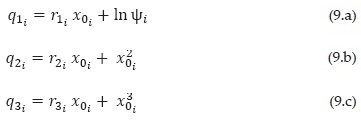

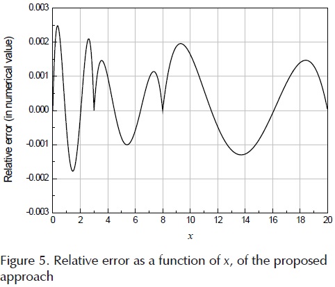
ψi=ψ (x0i) and ψi+1=ψ(x0i+1) and values are specified in Table 1, which are related to the corresponding x0i and x0i+1 values. For the first segment, the values of c01 and ψ1 can be also obtained as c0i= ψ1= . The values of coefficients in Table 1 and the relations 7 to 10 satisfy that the values estimates of the distribution function be continuous. As shown in Figure 5, the relative errors are lower than |εR (x) < 2.5 × 10⁻³|, which means that are below 0.25%. The relative errors associated to x values of 0, 3, 8 and 20 are equal to zero, which is consistent with the proposed approach. The error is greater than that obtained by (Rosenblueth, 1985) for one order of magnitude. The absolute error is lower than |εA (x) < 9.5 ×10⁻⁷ for x < 3, and its lower than |εA (x) < 6.4 ×10⁻⁴| for x ≥ 3. Figure 6 , shows that the proposed approach is good enough to adequately describe the function ψ(·). Besides, as is shown in the next section, the set of functions in Eq. (6) has the great advantage of being invertible.

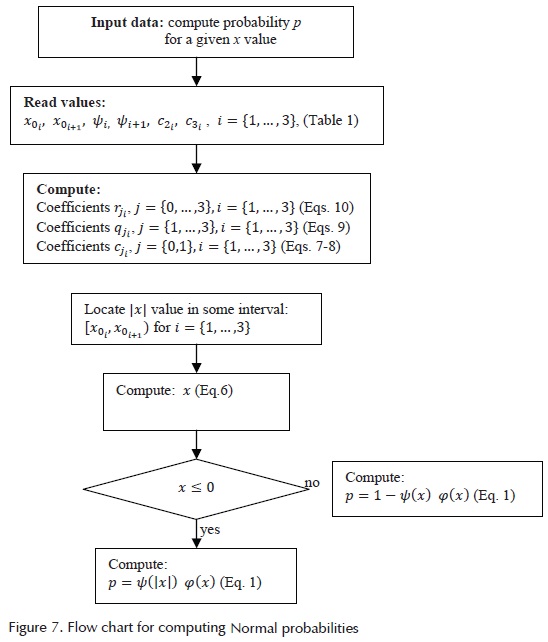
The generic flow chart shown in Figure 7 can be implemented in a computer program. The purpose is to describe the steps to compute a Normal probability value for a given value of the variable. If a number of computing is necessary, the coefficients need no further evaluation.
Inverses of normal probabilities
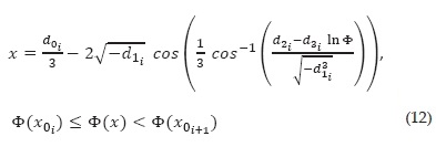
According to the last section, function ψ (·) can be described in three contiguous segments by means of functions ψ0i (·), i = {1, 2, 3}, given by Eq. (6). The inverse of Eq. (1) can be expressed as

and it can be computed as follows
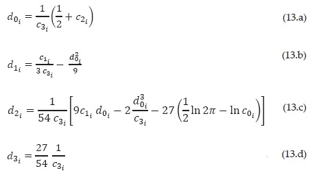
The parameters dji, j = {0, 1, 2, 3}, of each segment i are obtained in terms of the coefficients cji, j = {0, 1, 2, 3} of the corresponding segment i, by means of the expressions
Given that the coefficients dji and cji, j = {0, 1, 2, 3} are linked by means of expression 11, the x values correspond to a specific Φ (-x), which means that the numerical correspondences between these values is one to one (bijective).
The generic flow chart shown in Figure 8 can be implemented in a computer program. The purpose is to describe the steps to compute the inverse normal value for a given probability. This algorithm can be used alternatively to the algorithms described by (Knut, 1997 ) to simulate values of the Normal distribution. If a number of calculation is necessary, the coefficients no need further evaluation.

Conclusions
This work has proposed simple expressions that allow computing normal probabilities, even in the tail of the distribution, and their corresponding inverses. Such expressions are impressively manageable and useful for engineering applications. The proposed approach is simple because the resulting mathematical expressions are simple too, and its relative errors of the new approximation are lower than |εR (x) < 2.5 ×10⁻⁷| over a wide range of the random variable. The absolute error is lower than |εA (x) < 9.5 ×10⁻⁴| for x < 3, and its lower than |εA (x) < 6.4 ×10⁻⁷| for x ≥ 3. The approach does not have the inconveniences of typical approximations used in several applications that lead to relatively small absolute errors but significant relative errors, which become important in the tail of the probability distribution and are difficult to invert. Relative errors are critical when accurate estimations of small probabilities are required, so this new approximation is a powerful tool to compute probabilities or/and their inverses in engineering applications.
References
Abramowitz M. and Stegun I.A. Handbook of mathematical functions, 10th ed., New York, Dover Publications, 1972, 925-976. [ Links ]
Knuth D.E. The art of computer programming, Vol. 2, Seminumerical algorithms, 3th ed., Addison-Wesley, 1997, pp. 1-764. [ Links ]
Ordaz M. A simple approximation to the Gaussian distribution. Structural Safety, volume 9, 1991: 315-318. [ Links ]
Patel J.K. and Read C.B. Handbook of the normal distribution, Statistics Textbooks and Monographs, 2nd ed., New York, CRC Press, 1996, 1-427. [ Links ]
Rosenblueth E. On computing Normal reliabilities. Structural Safety, volume 2, 1985: 165-167. [ Links ]
Vedder J.D. An invertible approximation to the normal distribution function. Computational Statistics & Data Analysis, volume 16, 1993: 119-123. [ Links ]
Citation for this article:
Chicago style citation
Alamilla-López, Jorge Luis. An approximation to the probability normal distribution and its inverse. Ingeniería Investigación y Tecnología, XVI, 04 (2015): 605-611.
ISO 690 citation style
Alamilla-López J.L. An approximation to the probability normal distribution and its inverse. Ingeniería Investigación y Tecnología, volumen XVI (número 4), octubre-diciembre 2015: 605-611.
About the author
Alamilla-López Jorge Luis. The author is a civil engineer with master and doctorate degree in engineering from UNAM. He is a full-time researcher at the Mexican Petroleum Institute and teacher of postgraduate course in civil engineering at the School of Engineering and Architecture of the National Polytechnic Institute. He is at Level 2 in SNI (National System of Researchers). His main area of interest is focused on the modeling and assessment of the uncertain mechanical behavior of structural systems, on the stochastic modeling of loads and natural degrading phenomena, natural hazards, and on decision-making risk analysis. He published more than twenty papers in refereed journals.

