


 nueva página del texto (beta)
 Inglés (pdf)
 Artículo en XML
 Referencias del artículo
 Enviar artículo por email
 Citado por SciELO
  Similares en
SciELO
Similares en
SciELO 
 Permalink
1 Introduction
The fields of human-computer interaction and human-robot interaction aim to create natural and intuitive communication methods so that users can effectively give orders or share information with these machines.
One of the goals is to enable emotional interaction since humans are social beings who naturally seek emotional feedback from their conversational partners and convey information through their mood [4].
Emotion recognition in audio methods promises potential applications in the health sector and many other commercial applications. For instance, phycological therapy may offer an alternative and impartial opinion for a patient emotional state that the specialist can use to bring a better diagnosis.
Also, it can be used to track a patient’s emotional state over long periods; for commercial applications, it can be addressed to evaluate the user’s response to a product or service, which eases market research.
In cognitive sciences, the area that has carried out the most studies on emotion detection is Psychology. Multiple models have been proposed to try to understand emotions’ functioning and the relationship between them. Currently, no complete model can universally indicate the relationship between the different emotions; we still need to understand in depth the phenomenon that generates them since these relationships change from individual to individual.
There are two conceptual maps used mainly in computer sciences; the arousal-valence space [18, 20] and the categorical ones [10], and the main reason resides as they can easily be represented computationally. At the same time, they have demonstrated their validity in practical cases.
It is a widely accepted notion that the more input data, such as audio, video, speech, and posture, you process, the better detection and categorization you can achieve. However, adding more variables can complicate the classifier’s job, which presents a significant challenge, particularly when databases are limited in size. Due to the limited mobility and potentially invasive nature of sensors, most classifiers have concentrated on utilizing audio and video databases for their applications.
This article has considered evaluating the performance of three bioinspired classification systems on audio databases to compare their characteristics and identify the advantages and disadvantages of each one for this specific problem to guide future developments within the area.
The rest of the paper is organized as follows. In section 2, the main characteristics of the three types of neural networks are discussed.
Also, the emotion recognition problem is proposed. In section 3, the methodology implementation in some neuronal networks is addressed. In section 4, the results of the comparison are shown. In section 5, results are discussed, and future work is proposed.
2 Theoretical Framework
Many classifiers base their operation on the observed behavior of living beings, also called bio-inspired models. In this paper, three bio-inspired classifiers based on artificial neural networks were selected.
Firstly, spiking neural networks (SNN) participate in this comparison analysis due to closed similarities with biological neural networks, as they are the basis of future neuromorphic computer platforms. Neuromorphic computing seeks to emulate the behavior and structures present in the human brain for information processing.
In SNN realizations, it is possible to integrate into a single silicon die memory and process that presents power consumption of milliwatts, with parallel processing capabilities and integration levels of thousands of neurons.
As memory elements, memristors usually play a crucial role because they can adjust and maintain their electrical resistance based on the history of voltage and electrical current that has been applied between their terminals.
This ability to adjust and retain its resistance value can be used to store information and, therefore, to build non-volatile memories, playing the role of neural synapses [7, 8].
On the other hand, convolutional neural network models and their variants with recurring stages are the models that currently have the best results with this classification problem, mainly due to their ability to extract features from the data automatically.
Finally, MLP were examined, these models have been widely used to solve this classification problem, and currently, their variants are widely used as part of the models with convolutional layers.
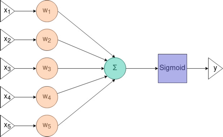
2.1 MLP
A Vanilla neural network, also known as a multi-layer perceptron (MLP), is made up of multiple layers of Perceptrons. These layers are connected through weights that multiply the inputs to them.
Each neuron perceptron performs the weighted sum of its inputs which serves as input to an activation function, usually a sigmoid one, relu, or tanh function. The output of this function is then evaluated against a threshold. If the value is greater than the threshold, the output is activated. The final neuron value is propagated to the next layer.
The reference [14] shows this model is a universal function approximator. Its popularity is due to its ability to be trained using an optimizer or the backpropagation algorithm, which adjusts the input weights of the neurons.
The goal is to minimize the error function by calculating the gradient and reaching a global minimum. This application teaches the network by providing it with a variety of examples and their corresponding expected outputs.
The backpropagation algorithm, then uses this information to adjust the weights of the inputs, reducing the error until it is minimal. However, be aware that overtraining can occur if the error is constantly reduced, causing the classifier to lose the ability to generalize.
2.2 CNN
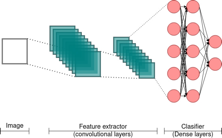
Convolutional neural networks, commonly known as CNN, have input layers comprising of convolutional neurons and output layers consisting of fully connected perceptrons, also known as dense layers. There are various models that utilize convolutional neurons, including full convolutional networks (FCN).
These networks are specifically designed to analyze images and extract features from them through convolutional layers. Each convolutional neuron generates a map of features, which is essentially a compressed version of the original image.
During training, the convolutional neurons act as filters that adjust their values, and the features that are extracted, become abstract representations after passing through multiple layers.
Although difficult to interpret for humans, these abstract representations contain the characteristics necessary for the dense layers to produce the best results. One advantage of this model is that feature extraction is handled by the convolutional layers, but a significant amount of training examples are required.
2.3 SNN
The Spiking Neural Networks model is based on the study of giant squid neurons by Hodgkin-Huxley (HH) [13] and aims to mimic biological neurons more closely.
Its primary purpose is to study biological systems rather than pattern recognition applications. The mathematical model includes four differential equations, making it computationally expensive.
To use these models as classifiers, simpler versions were proposed.
The leaky integrate and fire model (LIF) [1], for example, seeks to simplify the original model, while the Izhikevich model [15] is an intermediate interpretation that balances the simplicity of the LIF with the computational power of the HH model.
The Izhikevich model uses only two differential equations. There are different ways to train this type of neural network.
However, in the particular case of Izhikevich, its very nature prevents it from being trained using backpropagation methods, leading to problems during implementation since the optimizers usually have a higher computational cost.
Also one of the main characteristics of this type of neural network consists as it receives a signal as input, which must meet a series of characteristics, so an encoder must be created which converts the input data into spiking signals so that they can be learned by the network [17].
2.4 Recognition of Emotions in Audio
Various input data types can be considered to accurately identify emotions, including EEG [21] and posture.
It is believed that incorporating multiple cues, such as tone of voice and gesticulation, will improve the reliability of emotion classification.
While there are many possible inputs, practical approaches prioritize audiovisual data as it is less invasive and can be used in various environments to interact with the device properly. The context in which gestures occur can affect how classifiers interpret data. This is because different cultures and situations often lead to different interpretations.
Additionally, emotions can be subtle and sporadic, and people may hide them during small talk, making classification even more challenging.
When classifying emotions in audio, three types of databases are typically used. The first type involves using actors in controlled conditions, which has produced the most successful results with classifiers.
However, this database may not reflect real-life situations since the acted emotions are usually more exaggerated than genuine ones. The second type involves recording real emotions in controlled environments, attempting to capture emotions similar to those displayed in natural interactions.
These databases often produce fewer accurate results than the first type and can be difficult to create due to legal reasons or obtaining reliable data. Finally, the third type of database searches for audio samples that closely resemble what a classifier would encounter in the field, including multiple voices and background noise.
These databases are known as the wild [6] [9]. Audio databases for emotions are typically labeled in two ways, as previously mentioned. The first method involves an arousal-valence space map, which can help locate a particular emotion based on where these values fall.
The purpose of these maps is to represent the current understanding in cognitive science regarding emotions, with an emphasis on finding similarities. However, these maps also change from person to person, and although we can locate a more or less approximate parameter for various emotions, these are not static.
The second method of categorizing audio samples is by their corresponding emotion. This method is practical and straightforward, and is commonly used in audio emotion databases. Labels used for this method usually include the seven basic emotions, but some applications may use more complex labels.
To guarantee precision, creating a database of the possible examples the classifier can consult in specific applications is important.
3 Methodology
Even though the compared methods are different, we can still gain insights into how they work and how they can be used. This will enable us to identify useful characteristics that can help recognize emotions in audio and determine which model offers the most significant advantages.
3.1 Databases and Data Entry
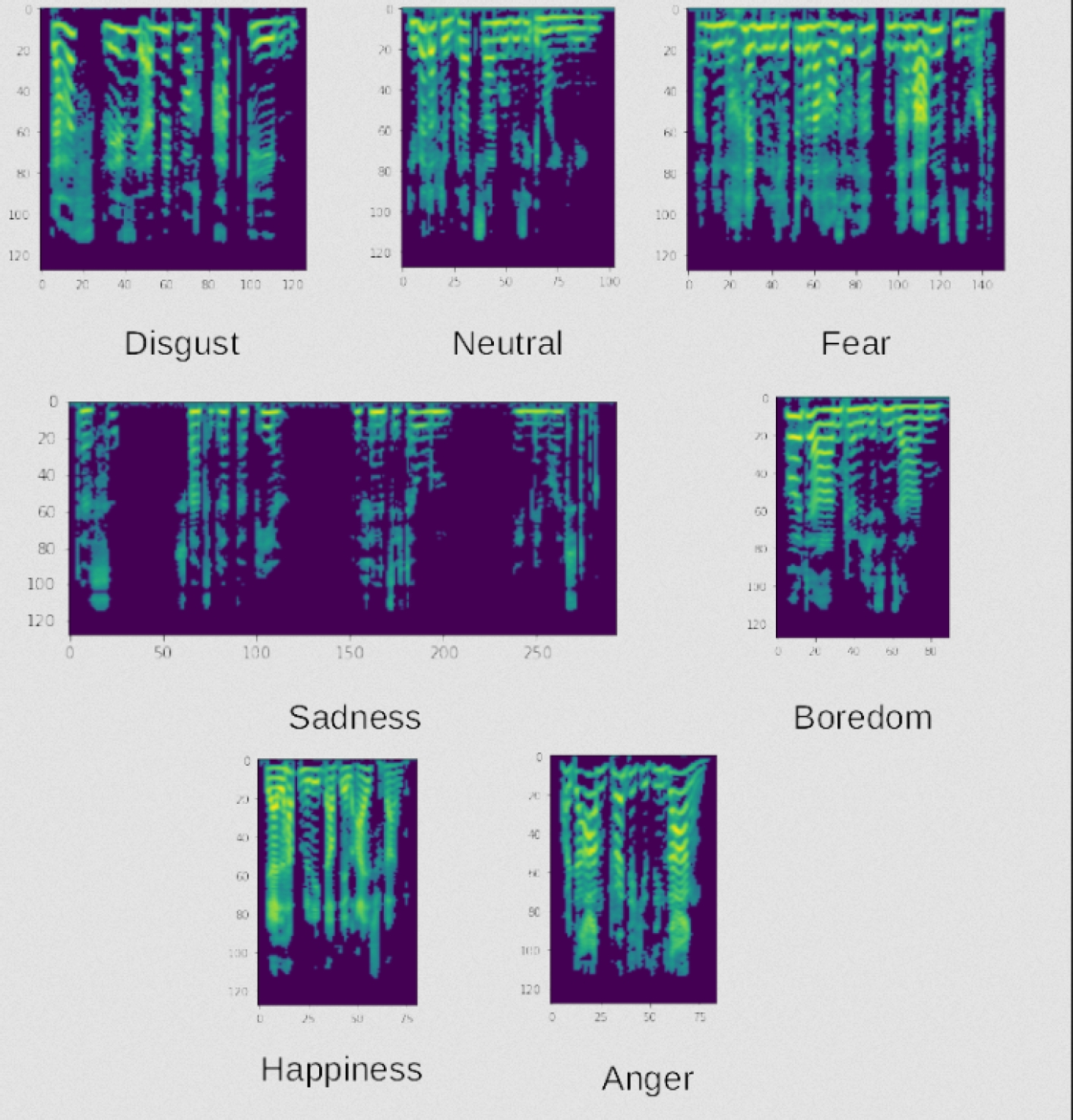
Three databases were used, which contain audio samples and are labeled with basic emotions, although there are differences in labeling between these sets, all three use basic emotions. One of the available databases for emotional speech analysis is EmoDB [5], created by the Institute of Communication Science at the Technical University in Berlin, Germany.
This database includes recordings from 10 actors (5 men and 5 women) expressing emotions such as anger, boredom, anxiety, happiness, sadness, disgust, and neutrality. It contains a total of 535 audio samples in German, although it is not a balanced database, this is the first database we employed.
The second is SAVEE [12] (Surrey Audio-Visual Expressed Emotion), which consists of 480 recorded audios of 4 male students between 27 and 31 years, with the categories anger, disgust, fear, happiness, sadness, and surprise.
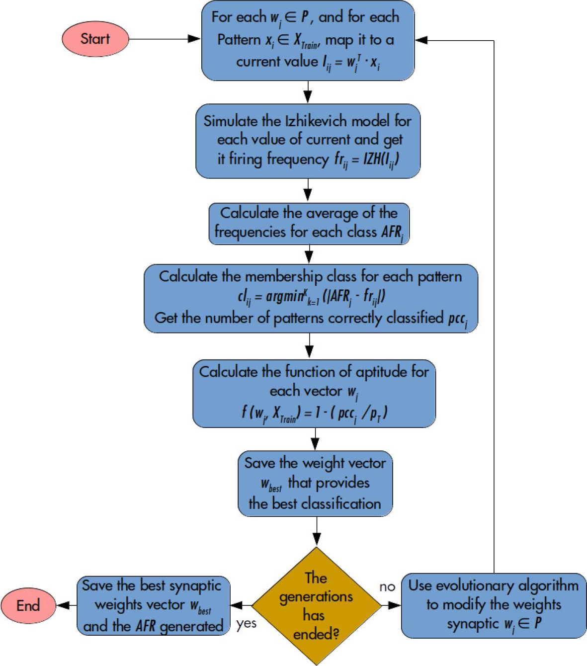
Fig. 5 Training method for SNN proposed in the Thesis ”Clasificación eficiente de patrones usando una sola neurona artificial” [3]
We also used RAVDESS [16], which is the Ryerson Audio-Visual Database of Emotional Speech and Song, to obtain 1440 speech audio files generated by 24 actors. These files have eight emotional categories, including neutral, calm, happy, sad, angry, fearful, disgust, and surprised.
From the speech audio, we identified various emotional features and discovered that the Mel-Spectrogram was the most effective for emotion perception. To minimize noise, we eliminated any values below 30 dB.
The Mel-Spectrogram is an audio analysis that enhances the Fourier spectrogram to accentuate low frequencies, which are more perceptible to the human ear.
3.2 Characteristics and Implementation of the SNN
We created our own model for the SNN because due to the lack of any existing models in the literature that used this type of neural network for emotion classification in audio.
To use the SNN for this purpose, an input signal must be provided, usually generated by an encoder that processes the available data. However, creating an effective encoder depends on the specific problem at hand.
In the case of emotions in audio, the lack of clear understanding of emotions in audio, makes it challenging to develop an effective encoder for the signal. When it comes to the input data generated by the encoder for these neural networks, specific characteristics must be met for the network to function properly.
Specifically, the signal must consist of pulses, as stated in [17]. Attempting to use an audio signal that has yet to be encoded beforehand will lead to unsatisfactory performance by the classifier.
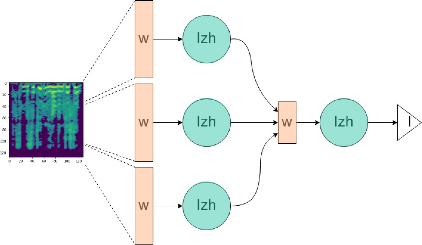
The architecture utilized in this project involves two layers of spiking neurons based on the Izhikevich model, chosen for their superior computing abilities [15]. The first layer is comprised of three neurons, receiving input from three vectors containing features extracted from the first column of the mel-spectrogram.
This window of 128 values represents the power of various frequencies in the audio and is divided into two vectors of 43 components and one of 42. Each vector undergoes a dot product with a set of weights to produce a single value for each neuron, representing a signal for a point in the input signal.
This process is repeated for the entire audio sample, generating the required input signal for the network to function.
To generate the signal that enters the second layer, the same process is followed as in the first layer. This generates a vector with the outputs of the first layer. The signal at the output of our neural network is then used to determine the class it belongs to, which is identified by its frequency. This type of neural network intrinsically has the quality of being recurrent, which is one of its main advantages.
However, as we can see in the SNN equation [15], this model requires a series of differential equations, increasing its computational complexity and computation time, while limiting the training methods:
The previous set of equations describes the Izhikevich neuron model. In equation 1,
In Equation 2,
We tested various optimization methods in order to train this neural network and found that the differential evolution approach (DE) provided the best results, even though it took the longest to optimize.
We also tested particle swarm optimization (PSO) and cybernetic optimization by simulated annealing (COSA) methods [11], with COSA being the quickest to converge but not as accurate as the DE.
This type of neural network requires mapping the output signal to a label. For this, the training methodology proposed in the thesis ”Clasificación eficiente de patrones usando una sola neurona artificial” [3] was utilized.
This methodology involves several steps. Firstly, the weights are initialized randomly. Next, the output frequency is obtained for each data point. Then, the average frequency per class is calculated.
After this, the relevance of each element to its corresponding class is evaluated to calculate the error. The values of the weights and parameters of the neurons are saved before proceeding to optimization.
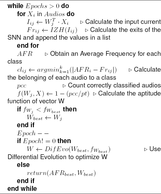
The process is then repeated from the second step. At the end, the weights, parameters of the networks, and frequencies of belongings that gave better results are saved. This method helps to assign labels to frequencies, but it may increase computation time.
It is clear that software implementation of these models requires more computing power, making them less efficient than models such as MLPs or CNNs.
Additionally, their implementation process is more complex. However, their unique nature is advantageous because they can be implemented in hardware by performing the differential equation using memristors, which has attracted the interest of numerous research teams.
One of the biggest challenges in using this model to classify emotions is the absence of an encoder. Currently, there isn’t enough knowledge about how emotions are expressed in audio to create one. This is a complex issue that must be addressed separately.
3.3 Characteristics and Implementation of the MLP
The MLP has been a popular classifier model, but in recent years, it has been overtaken by deep neural networks as the primary bio-inspired classifier.
According to a mathematical proof [14], an MLP can function as a universal function approximator. While it is true that a single hidden layer with n neurons can solve any decision boundary, this has led to misunderstandings and even caused the second winter of neural networks.
It is important to note that while one hidden layer can approximate any decision boundary, complex problems may require a large number of neurons. Additionally, the necessary database may be impractical to generate or the training time may exceed the age of the universe.
Perceptrons, being the basic element in an MLP [19], have the advantage that they use simple operations, ”adds and compares”, and activation functions with output in a defined range.
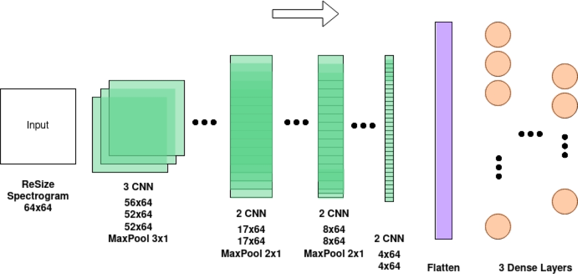
To prepare the data for input for the MLP, the spectrogram was resized to a fixed size of
However, because the MLP cannot extract features, a data expert must clean the data and create the necessary extractors for proper functionality. In this instance, the Mel-Spectrogram serves as the feature extractor generator.
The architecture used consisted of an input layer, 8 intermediate layers, and an output layer. Each intermediate layer had 500 neurons in a fully connected configuration, and the output layer had several neurons equal to the number of classes.
The training process involved using backpropagation, and labeling was done through one-hot coding. This approach is faster compared to metaheuristic methods.
Note that to simplify the training process for the network, more layers can be added to increase abstraction levels. This has been a known practice in MLPs and has led to the development of deep networks.
3.4 Characteristics and Implementation of the CNN
CNNs are designed to work on images; in this case, the image of interest is the audio spectrogram. The main characteristic that distinguishes this type of neural network is its ability to extract features from images, which is why they have become trendy for developing applications with complex input data, such as emotion detection.
Identifying emotions through this neural network requires many examples, but the databases are quite small, making it difficult. Data augmentation is commonly used to overcome this challenge, which was not used in this project.
In a typical CNN, the initial layer consists of convolutional neurons that work like image filters.
However, they are adaptable and aid in extracting image features, such as the Mel-spectrogram, by optimizing weights during training. These neurons learn which features the classifier needs and are often paired with a max-pooling and a batch normalization layer.
Convolutional layers produce feature maps that can be quite large. To reduce their size, we use max pooling layers. These layers retain the highest values in the feature maps and discard the lowest values using a kernel.
If the kernel size is 2, the feature map size is halved. While there are other types of pooling layers, such as Mean and Min pooling, they are not as frequently used.
During the training process, batch normalization layers are utilized to decrease the variance of input values and speed up the convergence towards a minimal error.
Following the convolutional layers, a set of neurons resemble MLP, but utilize distinct activation functions. These neurons perform the classification task and are referred to as dense layers. During this phase, the neurons are fully connected, linking each neuron of one layer with every neuron in the next layer.
Finally, the process culminates in an output layer consisting of one neuron representing each class.
The table below describes the network’s architecture. Currently, the best performing models are convolutional neural networks with added recurrent capabilities, as noted in [2].
4 Results
To compare the performance of different models, we conducted tests simulations with three databases, each with 1,000 epochs. To ensure fairness, we balanced the databases by reducing the examples in each class.
We did not use data augmentation as our main goal was to evaluate the models rather than achieve the best classification.
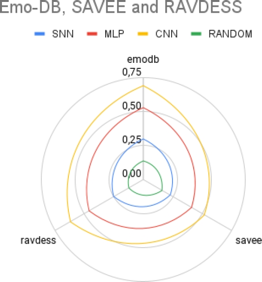
After balancing, EmoDB had 322 samples, SAVEE had 420, and RAVDESS had 768. The accuracy of each model is presented in the table below.
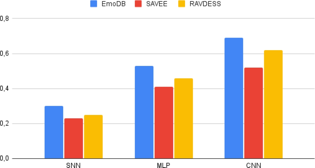
The following graphic displays the varying levels of accuracy achieved by different models. Out of the three databases, CNN performed the best overall. This is due to CNN’s ability to extract information from images.
It’s clear that the CNNs displayed the best performance. However, it’s worth mentioning that the SNNs had a longer training time and performed poorly compared to other models. It’s also worth noting that, that there are currently limited resources for creating and evaluating spiking neural networks.
As a classifier, the MLP demonstrates some effectiveness, considering that there are 7 classes and the expected accuracy for the Emo-DB dataset is around 14.25%. The experimental results show an average classification rate of 53%.
To summarize, the features of the suggested networks are evident in this issue. It is noticeable that all 3 models can classify with varying levels of success. This article highlights that SNNs have a smaller architecture compared to other models.
Even without an encoder, they produce better results than random selection. However, training time and computational complexity are limitations.
One advantage of SNNs is their ease of implementation in hardware, which has attracted the attention of research groups working towards practical parallel and low-power hardware implementations. Implementing SNNs in hardware could eliminate the above-mentioned limitations.
Even though the MLP is much larger and more computationally complex, it has a lower training time and better classification capacity compared to the SNN.
As previously stated, CNNs are renowned for their capacity to identify features and have exhibited the best performance. Nevertheless, they require many examples and epochs to attain precise learning. They are generally larger networks than traditional MLPs but have demonstrated success in multiple fields.
The results of the F-Score help to reveal in more detail the inner workings of the tested models for an specific problem, it also shows how certain classes are easier for the models to recognize.
In the case of the CNN, it can be seen how there are large variations in performance between each of the databases, in the case of EMO-DB we can see that there are classes whose classification is 0, in the case of the RAVDESS it’s seen there is a moderately balanced performance between all classes and in the case of SAVEE we see again there are classes that doesn’t seem to be classified but at the same time the classified ones show a better balance than EMO-DB, this could be due to the differences between data that each set has, which could be the language, quality or duration of the audios.
But in our experience with the experiments, we suggest that differences can be more influenced by the size of the databases, even if it is the case, we see there are emotions that are easier to detect than, emphasizing anger and happiness.
For the MLP performance was quite lower and shows how the results are concentrated in only a couple of classes, we see the lack of feature extraction plays a very big role in the performance of the network, we suppose this phenomenon happens since it stays at a local minimum.
Performance among the three databases also varies depending on the number of audio samples.
In the case of SNN, which show results with a balance similar to CNN but with lower performance, we believe this shows the network generates a certain extraction of features because this network doesn’t have an encoder.
As mentioned in previous sections, we think this is a large fraction of the problem for getting such a poor performance, but nonetheless, it’s quite interesting to see that there is some level of feature extraction.
5 Conclusions
By examining the key features of these bio-inspired models, we can gain insight into potential future approaches for enhancing audio emotion recognition. Refer to Table 3 for a comprehensive overview of the models’ main characteristics of this problem.
Table 1 CNN Layers
| Layer (type) | Output Shape | Param # |
| conv2d (Conv2D) | (None, 56, 64, 10) | 100 |
| conv2d 1 (Conv2D) | (None, 52, 64, 10) | 510 |
| conv2d 2 (Conv2D) | (None, 52, 64, 10) | 310 |
| max pooling2d (MaxPooling2D) | (None, 17, 64, 10) | 0 |
| batch normalization (BatchNo) | (None, 17, 64, 10) | 40 |
| conv2d 3 (Conv2D) | (None, 17, 64, 40) | 1240 |
| conv2d 4 (Conv2D) | (None, 17, 64, 40) | 4840 |
| max pooling2d 1 (MaxPooling2) | (None, 8, 64, 40) | 0 |
| batch normalization 1 (Batch) | (None, 8, 64, 40) | 160 |
| conv2d 5 (Conv2D) | (None, 8, 64, 80) | 32080 |
| conv2d 6 (Conv2D) | (None, 8, 64, 80) | 6480 |
| max pooling2d 2 (MaxPooling2) | (None, 4, 64, 80) | 0 |
| batch normalization 2 (Batch) | (None, 4, 64, 80) | 320 |
| conv2d 7 (Conv2D) | (None, 4, 64, 80) | 6480 |
| flatten (Flatten) | (None, 20480) | 0 |
| dense (Dense) | (None, 80) | 1638480 |
| dense 1 (Dense) | (None, 30) | 2430 |
| dense 2 (Dense) | (None, 7) | 124 |
Table 2 Model’s Accuracy
| . | EmoDB | SAVEE | RAVDESS |
| SNN | 0.3 | 0.23 | 0.25 |
| MLP | 0.53 | 0.41 | 0.46 |
| CNN | 0.69 | 0.52 | 0.62 |
Table 3 F-Score EmoDB
| . | Anger | Boredom | Disgust | Fear | Happiness | Sadness | Neutral |
| SNN | 0.0 | 0.1 | 0.05 | 0.0 | 0.1 | 0.07 | 0.0 |
| MLP | 0.15 | 0.0 | 0.0 | 0.1 | 0.23 | 0.0 | 0.0 |
| CNN | 0.0 | 0.2 | 0.15 | 0.0 | 0.7 | 0.45 | 0.21 |
When we consider the traits of the suggested models, it is evident that combining CNNs and recurrent models with data augmentation techniques leads the way in emotion recognition.
However, this also establishes a minimum requirement for computational power that platforms using them must meet to be considered for emotion recognition applications.
This can be a challenge for low-cost robots intended for commercial applications that focus on human-robot interaction.
Table 4 F-Score SAVEE
| . | Anger | Disgust | Fear | Happiness | Neutral | Sadness | Surprise |
| SNN | 0.04 | 0.01 | 0.15 | 0.01 | 0.1 | 0.26 | 0.1 |
| MLP | 0.25 | 0.0 | 0.0 | 0.21 | 0.0 | 0.0 | 0.12 |
| CNN | 0.36 | 0.0 | 0.2 | 0.24 | 0.0 | 0.38 | 0.30 |
Table 5 F-Score RAVDESS
| . | Neutral | Calm | Happy | Sad | Angry | Fearfull | Disgust | Surprise |
| SNN | 0.11 | 0.04 | 0.08 | 0.1 | 0.23 | 0.07 | 0.01 | 0.15 |
| MLP | 0.4 | 0.0 | 0.48 | 0.0 | 0.51 | 0.0 | 0.0 | 0.0 |
| CNN | 0.43 | 0.42 | 0.18 | 0.2 | 0.64 | 0.47 | 0.46 | 0.40 |
Table 6 Characteristics
| . | Information extraction | Computational Complexity | Training time |
| SNN | Yes, poorly | Is the most complex | Requires more time than the others |
| MLP | No | Is the less complex | Requires less time than the others |
| CNN | Yes | . | . |
5.1 Future Work
Another interesting proposal involves the use of spiking networks implemented in hardware. This approach aims to eliminate the main drawbacks of these models.
However, the main challenge remains -designing an encoder that can convert emotions into spiking signals. As a more practical alternative, CNNs must be utilized as extractors for the spectrogram to serve as an encoder capable of learning the optimal values to activate the SNN.

