


 nova página do texto(beta)
 Inglês (pdf)
 Artigo em XML
 Referências do artigo
 Enviar este artigo por email
 Citado por SciELO
  Similares em
SciELO
Similares em
SciELO 
 Permalink
1 Introduction
Numerical models of the atmosphere, based on initial meteorological data, apply physical-mathematical models to calculate the future state of meteorological variables such as relative humidity, temperature, precipitation, wind speed and direction, among others. With the advancement of computing and knowledge of the atmosphere, these models have evolved and correspond to the first consultation reference in operational forecasting centers. Among the input data, the models consider the geographical characteristics of the study área, among which are the topography, Coriolis force, angle of rotation of the earth and definition of type of land use. The latter allows an appropriate representation of processes related to the radiation balance and the local hydrological cycle [8].
The WRF (Weather Research and Forecasting) model has become the most widely used in the scientific community with more than 57,800 users from 160 countries [23]. This model was developed by different institutions in the US, including NCAR (National Center for Atmospheric Research), NCEP (National Centers for Environmental Prediction) and NOAA (National Oceanic and Atmospheric Administration). The main characteristics of the model revolve around its non-hydrostatic dynamics and its ability to operate in spatial resolutions of a few kilometers.
Contains different configuration options and physical parameterizations for convection, microphysics, planetary boundary layer, radiation, among other hydrothermodynamic processes.
The model code is open to the community and has been optimized for operation in both shared and distributed memory computing environments [3, 30].
The WRF model uses by default a classification of 21 categories of land use type, defined in the International Geosphere and Biosphere Program (IGBP), based on MODIS satellite images between 2001-2005 and a resolution of 500 meters [7]. However, over the years, naturally or by anthropogenic effect, there are changes in the type of land use in specific áreas, for example, the transfer of grasslands and scrublands to agricultural uses [33], so the default database is not considered current or applicable to recent events or several years prior to its creation.
On the other hand, remote sensing is fundamentally based on the fact of working with descriptive information of phenomena and objects present in the physical universe that has been collected without coming into contact with them, making it a very efficient alternative for remote monitoring [17]. Remote sensing makes it possible to explore various aspects of our planet in different spectral bands.
For example, through remote sensing it is possible to identify changes in vegetation cover and bodies of water, types of climates, advance or retreat of glaciers, felling of forests, erosion processes, among others [20, 34]. In addition to the direct use of the different spectral bands, derived spectral indices have been developed, which allow to improve the identification of characteristics or objects that are not directly identifiable from the satellite bands [1, 10,29].
The objective of this work was to apply a methodology for the classification of types of land use in the Metropolitan Zone of the Valley of Mexico based on the analysis of the spectral signature of Landsat 8 Satellite images and derived indices to later replace the default database of the WRF model and statistically evaluate its effect on the precipitation simulation for a selected event with extraordinary rainfall in the year 2020.
2 Metodology
2.1 Study Zone
The Metropolitan Zone of the Valley of Mexico (ZMVM or Valley of Mexico) is located at 19°20’ North Latitude and 99°05’ West Longitude, in the center of the country, forming part of a basin, which has an average elevation of 2,240 meters above sea level (masl); it presents intermountain valleys, plateaus and ravines, as well as semi-flat terrain, in what were once the lakes of Chalco, Texcoco and Xochimilco [30]. The ZMVM is the main economic, financial, political and cultural center of Mexico. With respect to its population, it is the third largest metropolitan área in the Organization for Economic Cooperation and Development (OECD) and the largest in the world outside of Asia. According to the most used Mexican delimitations, the ZMVM covers around 9,560 km2 (almost five times the size of the Greater London region and three times that of Luxem-bourg), includes the 16 delegations of the Federal District, 59 municipalities of the state of Mexico and one municipality of the state of Hidalgo [26].
2.2 Datasets
2.2.1 Meteorological Fields
To generate the initial and boundary conditions required by the WRF model, data from the Global Tropospheric Analysis System of the NCEP FNL (Final) operational model were used, which operates from the month of July 1999 [24]. The FNL data was downloaded from the 7th at 00:00 until the 9th of June at 18:00 of the year 2020, in UTC time (Universal Time Coordinated). These data are in GRIB format with a temporal resolution of 3 hours and a spatial resolution of 27 km.
2.2.2 LANDSAT Satellite Images
For the analysis of the spectral signature, the images of the Landsat 8 satellite, launched into space in August 2012, were used. Contains 11 bands with an average resolution of 30 m, which allows a wide range of applications. The consultation, download and cropping of the images was carried out by means of Google Earth Engine (GEE), tool developed by the company Google that allows geospatial analysis to be carried out using processing and data collections in the cloud [27].
Using GEE’s Javascript code editor, the process of selecting, cutting and downloading the images for the ZMVM in Tiff format was automated. Four images were selected for the year 2020, one per season of the year, applying as the main criterion the selection of images without the presence of clouds that could affect the classification. The values of the 11 bands were normalized on a scale of 0 to 1.
2.2.3 Rainfall Records
As observed data, the daily rainfall records of the weather stations of the Hydrological Information System (SIH) were used, operated by the Surface Water and River Engineering Management (GASIR) of the National Water Commission (CONAGUA). The data from these stations correspond to the accumulated rainfall from 6:00 hours of the day before to 6:00 hours of the day of registration.
For this study, only the data reported for June 9, 2020 was used, being a total of 82 weather stations that contained data in the study área. The maximum precipitation reported for this date was 63.5 mm at the station “Las arboledas” with ARBMX station key, latitude 19.5667, longitude -99.2167 and an elevation of 2,280 masl.
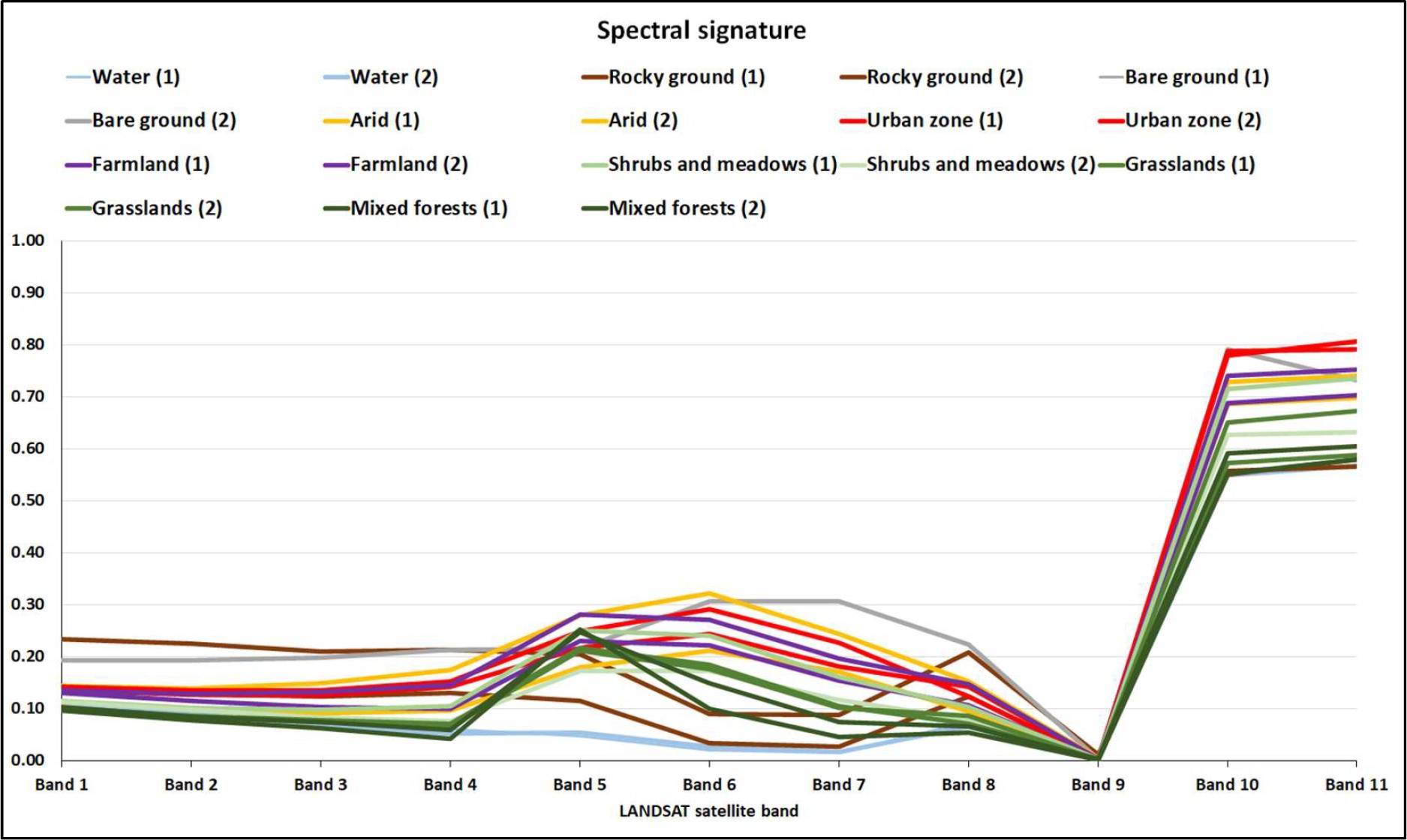
2.3 Analysis of the Spectral Signature
The analysis of the spectral signature and derived indices was carried out to identify 10 types of land use: arid soil, bare ground, farmland, grasslands, snow, mixed forests, rocky ground, shrubs/meadows, urban zone and water. The selected spectral indices are described below.
The Normalized Difference Building Index (NDBI), allows estimating built-up surfaces or construction development [4, 35]. It is expressed in values from -1 to 1. Positive values indicate áreas built up or under construction, while negative values indicate áreas with vegetation or bare soil (Eq. 1):
where NIR correspond to near infrared (band 5 on Landsat 8) and SWIR correspond to shortwave infrared (band 6 on Landsat 8).
The Normalized Difference Vegetation Index (NDVI), identifies presence of vegetation [29]. It is expressed in values from -1 to 1 (Eq. 2). Values greater than 0.2 indicate áreas with vegetation, while opposite values indicate urban áreas, arid soils, among others:
where Red corresponde to visible red (band 4 on Landsat 8) and NIR correspond to near infrared (band 5 on Landsat 8).
The Urban Index (UI), allows estimation of built-up áreas [14]. It is expressed in values from -1 to 1. Where positive values indicate urbanized áreas, while negative values refer to bare or vegetated áreas (Eq. 3):
where SWIR correspond to shortwave infrared 1 (band 6 on Landsat 8) and VNIR correspond to shortwave infrared 2 (band 7 on Landsat 8).
The Normalized Difference Snow Index (NDSI). It is expressed in values from -1 to 1. Where values close to 1 indicate áreas with ice or snow (Eq. 4):
where Green correspond to visible green (band 3 on Landsat 8) and SWIR correspond to shortwave infrared 1 (band 6 on Landsat 8).
The Normalized Differential Water Index (NDWI), allows to identify water masses and áreas saturated with moisture [5]. It is expressed in values between -1 and 1. Positive values indicate bodies of water, flooded or humid áreas, while negative values indicate dry áreas (Eq. 5):
where Green correspond to visible green (band 3 on Landsat 8) and NIR correspond to near infrared (band 5 on Landsat 8).
Subsequently, the spectral signatures were generated for two points, randomly selected, for the types of land use defined, with the exception of the snow category because no pixels were found in the treated images.
Significant variations were observed during the year in the categories of vegetation cover and bodies of water; therefore, it was determined to make an average of the images corresponding to the four seasons of the year, determining the spectral signature on these values.
Figures 1 and 2 present the spectral signature by type of land use by band and by spectral index respectively.

Based on the bibliography and on the analysis of both the spectral signature and the derived indices, it was possible to define a classification of 10 categories of land use types called LANDSAT classification.
The NDVI allowed a clear distinction to be made between the categories with vegetation from the rest, therefore it was determined that this index can be used as the first classification filter, but not determining, since some types of soil, such as arid soil, farmland and urban áreas presented values in the same range.
For these categories, the values of other indices and specific bands are considered. Table 1 presents the LANDSAT classification and the key values for its detection.
Table 1 Land use type categories identified based on the spectral signature and indices derived from the LANDSAT satellite
| Index | Land use | NDVI value | Other values |
| 1 | Water bodies | <= 0.0 | NDWI >= 0.1 |
| 2 | Snow | NDSI >= 0.9 | |
| 3 | Rocky ground | ||
| 4 | Bare ground | <= 0.10 | |
| 5 | Arid soil | <= 0.25 | |
| 6 | Urban zone | Band 10 >= 0.75 Band 11 >= 0.75 UI >= 0.05 NDBI >= 0.05 |
|
| 7 | Farmland | <= 0.4 | Band 1 >= 0.1225 Band 2 >= 0.1069 |
| 8 | Shrubs and meadows | ||
| 9 | Grasslands | <= 0.6 | |
| 10 | Mixed forest | > 0.6 |
Subsequently, a relationship was created between the 21 categories of land use type that the WRF model uses by default (MODIS), and the 10 categories of the LANDSAT classification obtained from the previous analysis. Table 2 shows the LANDSAT classification indices and their equivalence in MODIS.
Table 2 Equivalence between land use type indices between the default database of the WRF model (MODIS) and the LANDSAT classification
| MODIS | LANDSAT | ||
| Index | Land use | Index | Land use |
| 1 | Evergreen needle-leaf forest | 10 | Mixed forest |
| 2 | Evergreen broadleaf forest | ||
| 3 | Deciduous Needle-Leaf Forest | ||
| 4 | Deciduous forest | ||
| 5 | Mixed forest | ||
| 6 | Closed scrub | 8 | Shrubs and meadows |
| 7 | Open scrub | ||
| 8 | Wooded savannahs | ||
| 9 | Savannahs | ||
| 10 | Grasslands | 9 | Grasslands |
| 11 | Permanent wetlands | 1 | Water bodies |
| 12 | Farmland | 7 | Farmland |
| 13 | Urban and build | 6 | Urban zone |
| 14 | Mosaic of farmland / natural vegetation | 7 | Farmland |
| 15 | Ice/Snow | 2 | Snow |
| 16 | Barren or sparsely vegetated | 3 | Rocky ground |
| 4 | Bare ground | ||
| 5 | Arid soil | ||
| 17 | Water | 1 | Water bodies |
| 18 | Wooded tundra | [Unclassified] | |
| 19 | Mixed tundre | [Unclassified] | |
| 20 | Barren tundre | [Unclassified] | |
| 21 | Lakes | 1 | Water bodies |
The steps to generate the LANDSAT classification are as follows:
Step 1. Open Geotiff file with the 11 bands of the LANDSAT satellite.
Step 2. Read the 11 bands into independent variables.
Step 3. Calculate the derived indices NDBI, NDVI, NDSI AND NDWI and UI.
Step 4. Obtain dimensions nx and ny of the satellite bands.
Step 5. Create the classification array of ny and nx dimensions.
Step 6. Iterate for each mesh point and assign the category to the variable classification according to the values of the table 1.
Step 7. Close Geotiff file.
The classification variable will be used in the process of updating the LU_INDEX variable of the file with the default geographic data of the WRF model.
It is necessary to point out that, for each category, here are values corresponding to the physical parameters of albedo, soil moisture availability, surface emissivity, roughness thickness, thermal inertia and surface heat capacity that considers the WRF model for each type of specific land use, these values are found in the LANDUSE.TBL file, included within the model file structure.
2.5 Updating the Land Use Type Layer
Once the LANDSAT classification has been obtained, with 30 m resolution, the values of the LU_INDEX variable of the original file were updated with the geographic data of the d02 domain (geo_em.d02) generated with the WPS (WRF Preprocessing System) module, the latter with a resolution of 1 km.
This process involves sampling all the points of the LANDSAT classification contained for each grid point of the variable LU_INDEX and assigning it the modal value. The WRF model uses an Ara-kawa-C type mesh [31], therefore, each grid point has geographic coordinates that correspond to the center (XLAT_M and XLONG_M), to the vertex V (XLAT_V and XLONG_V) and to the vertex U (XLAT_U and XLONG_U).
The steps for updating the LU_INDEX variable with the LANDSAT classification are as follows:
Step 1. Open the file with the geographic data (by default) of the domain d02 in NetCDF format (geo_em.d02), which were generated by the WPS module.
Step 2. Read the variables LU_INDEX, XLAT_U, XLONG_U, XLAT_V and XLONG_V.
Step 3. Get ny and nx dimensions of the variable LU_INDEX.
Step 4. Iterate y and x for each mesh point and update LU_INDEX according to the following:
Step 4.1. Obtain minimum longitude (lonMin) of vertex U (XLONG_U[y, x])
Step 4.2. Get maximum longitude (LongMax) of vertex U (XLONG_U[y, x+1])
Step 4.3. Get minimum latitude (latMin) of vertex V (XLAT_V[y, x])
Step 4.4. Get maximum latitude (latMax) of vertex V (XLAT_V[y+1, x])
Step 4.5. Find the indices iy1 and iy2 in the LANDSAT classification mesh within the vertices of the LU_INDEX cell corresponding to latMin and latMax.
Step 4.6. Find the indices ix1 and ix2 in the LANDSAT classification grid within the vertices of the LU_INDEX cell corresponding to lonMin and lonMax.
Step 4.7. Extract from the classification variable a subgrid of the segment [iy2:iy1,ix1:ix2] and store it in the tmp variable.
Step 4.8. Get the mode of the variable tmp.
Step 4.9. Replace LU_INDEX[y,x] with mode.
Step 5. Update the LU_INDEX variable in the file with the geographic data.
Step 6. Close the Geo file.
2.6 Rainfall Simulation with the WRF Model
For this study, the ARW (Advanced Research WRF) kernel was used in its version 4.2. This kernel allows horizontal nesting, making it possible to obtain a higher resolution in a specific área, this is achieved by adding one or more additional meshes or domains to the simulation. This option is for horizontal refinement, with rectangular meshes that are aligned to a coarser parent mesh called the parent domain (d01), within which subsequent meshes can be nested (d02, d03, etc.) called nested domains [18].
Among the good practices, it is recommended to scale down between the parent and nested domains from 1-3 or 1-5 to maintain stability in the model. For the simulation of rainfall in the ZMVM, the WRF model was configured for domains d01 and d02 with 5 and 1 km resolution, respectively, thus maintaining the relation 1-5.
Two numerical simulations were carried out to obtain the accumulated rainfall in 24 hours between June 8 at 6:00 hours and June 9 at 6:00 hours, same period of the observed data selected from the SIH database.
Simulations were performed with a 38 hours warm-up, the first using the MODIS default land use type and the second with the LANDSAT classification.
Although exact methods exist to solve small-scale physical processes, these are not considered appropriate for their application in numerical models because they require a long computation time and the meteorological values required for their calculation are not included in the required scale and quality.
So that, the WRF model uses different types of parameterizations to simplify processes that are too small and complex. Table 3 shows the main configuration parameters of the domains. Table 4 shows the parameterization schemes selected for this study.
Table 3 Configuration parameters of the domains of the WRF model
| Parameter | Description | Parent domain (d01) | Nested domain (d02) |
| i_parent_start | Starting Lower Left Corner I-indices from the parent domain | 1 | 27 |
| j_parent_start | Starting Lower Left Corner J-indices from the parent domain | 1 | 27 |
| e_we | End index in x (west-east) direction | 51 | 86 |
| e_sn | End index in y (south-north) direction | 51 | 86 |
| dx/dy | Grid length in x/y direction, unit in meters | 5000 | 1000 |
| Parent_grid_ratio | Parent-to-nest domain grid size ratio. | 1 | 5 |
| Lat_central | Real value with the central latitude of the parent domain. | 20.687 | Does not apply |
| Long_central | Real value with the central longitude of the parent domain. | -103.348 | Does not apply |
Table 4 Selected parameterization schemes in the WRF model
| Process | Parameterization scheme (for both domains) |
| Microphysics | Option 9: Milbrandt–Yau Double Moment Scheme [15, 16]. |
| Convection | Option 3: Grell–Freitas Ensemble Scheme [9]. |
| Planetary boundary layer | Option 5: Mellor–Yamada Nakanishi Niino Level 2.5/3 Schemes [21, 22, 25]. |
| Layer options surface | Option 1: Revised MM5 Scheme [13]. |
| Land surface options | Option 1: 5-layer Thermal Diffusion Scheme [6]. |
| Long wave radiation | Option 4: RRTMG Longwave Scheme [11]. |
| Short wave radiation | Option 4: RRTMG Shortwave Scheme [11]. |
| Urban surface options | Option 1: Single Layer Urban Canopy Model [4]. |
2.7 Statistical Evaluation
To measure the effect of updating the land use type layer on the rainfall simulation with the WRF model, the BIAS, MAE and RMSE statistics were applied between the observed rainfall and the simulated rainfall by the WRF model.
The BIAS measures the error that occurs systematically, so it is a good indicator to measure the reliability of the models [28]. It can be positive (overestimation) or negative (underestimation) (Eq. 6):
where N is the number of observations, Pi is the value of the model prediction in element i and Oi is the value of the observation in element i.
The Mean Absolute Error (MAE) is a widely used measure in model evaluations [2, 32]. Provides the average of the absolute difference between the model prediction and the observed value (Eq. 7):
The Root Mean Square Error (RMSE) expresses the total error of the model [32]. Consists of the square root of the sum of the squared errors, which captures both positive and negative errors; therefore, it expresses both systematic and random errors (Eq. 8):
3 Results
Significant variations were observed mainly in the category’s farmland and urban zone. Farmland in MODIS classification is minimal, this is considered wrong, since according to INEGI [12], the área for agriculture in the ZMVM amounts to 36%.
It should be considered that urban agriculture is not only within the city, but also on its edges, which have lost their agricultural tradition due to urban expansion. Urban agriculture in these áreas is the result of rural-urban migration, it is a practice that is recovered by the emigrated population with strong community roots towards their places of origin [19].
Regarding the urban zone, the LANDSAT classification detects urban growth in the north and northwest between the limits of the ZMVM and the state of Hidalgo.
However, in MODIS other classifications are considered as urban, therefore in km2 it presents a higher frequency.
Figure 3 shows the comparison between the MODIS and LANDSAT classification. Figure 4 shows the histogram of frequencies with both classifications. Figure 5 shows the comparison between the rainfall records from the SIH weather stations and those simulated by the WRF model with MODIS and LANDSAT.


Fig. 5 Accumulated rainfall (mm) in 24 hours observed, simulated WRF-MODIS and simulated WRF-LANDSAT
Finally, the statistical metrics were applied between the observed values and those simulated by the WRF model for the two simulations. In all the experiments negative BIAS values were obtained, this indicates that the model presents a systematic error with a tendency to underestimate, that is, at the comparison grid points, the model simulates less rainfall than what actually occurred in the ZMVM.
Regarding the MAE metric, this tells us that the expected average error ranges between 10.81 and 11.77 mm. On the other hand, RMSE presents a cumulative variance between 163.56 and 168.09.
However, according to the BIAS, MAE and RMSE metrics, an improvement was observed in the precipitation simulation with the LANSAT classification with respect to MODIS. Table 5 presents the results obtained with the statistical metrics.
4 Conclusions
The methodology presented allowed a classification of the types of land use predominant in the Metropolitan Zone of the Valley of Mexico. Each category can be obtained directly based on the spectral signature of the bands and the derived indices. It was identified that the NDVI can be used as the first classification filter, but not as a determinant, since some land use, such as arid soil, urban áreas and farmland present values in the same range, for these cases other indices and auxiliary bands should be used.
The main variation with the updating of the type of land use corresponds to the categories of urban zone and farmland in the Metropolitan Area of the Valley of Mexico. Although the MODIS classification mostly covers Mexico City, it omits some urban spots in the north and northwest that are identified in the LANDSAT classification. Regarding farmland, in the MODIS classification this is minimal, while the LANDSAT classification is considered more realistic. The substitution of the land use type layer on the original file generated by the WRF preprocessing module was transparent, so the numerical simulations were carried out successfully.
The effect on the simulation of the rainfall variable was evaluated for the storm reported by the SIH on June 9, 2020. With a maximum record of 63.5 mm at the “Las arboledas” station with ARBMX code, latitude 19.5667, longitude -99.2167 and an elevation of 2,280 masl. In general, it was observed that the model had a tendency to underestimate, however, there was an improvement in the precipitation simulation with the LANDSAT classification, this based on the statistical results that went from 9.36, 11.77 and 168.09 to -8.84, 10.81 and 163.56 of the BIAS, MAE and RMSE metrics respectively.
The variation in the rainfall simulation with and without updating the land use type layer highlights the sensitivity of the WRF model to the characteristics of the terrain.

