


 nueva página del texto (beta)
 Inglés (pdf)
 Artículo en XML
 Referencias del artículo
 Enviar artículo por email
 Citado por SciELO
  Similares en
SciELO
Similares en
SciELO 
 Permalink
1 Introduction
Protein complexes are compounded by several amino acid chains binding by non-covalent protein-protein interactions [28].
The Bone morphogenetic proteins (BMPs) are a group of similar-structure proteins with short-length amino acid chains and low molecular weight that configures functional growth factors presented in PPI zones [8, 33].
Identifying and classifying these zones, especially the amino acids that thermodynamically convey these interactions, are critical for developing new reaction mechanisms and discovering new drugs inside the Protein complexes [25].
For these reasons, our work is focused on this detection and classification, assuming that the ground-state energy of the amino acids is affected by their interacting zone.
This zone, in which these amino acids are located, is the PPI. The interacting zones between the chain in protein complexes are called interface residues, as shown in Fig. 1, which forms a region where two or more protein chains link themselves by non-covalent interactions such as Van der Waals, electrostatic, hydrogen bonding, ionic, and other forces [12].

Fig. 1 Interface residues of the 1M4U Protein Complex, which contains two chains (ribbon representation) code A (green) and code L (cyan), respectively. The interface residues of the interaction between them are represented by the red section (visualized using Pymol [34])
1.1 Hot Spots and Hot Regions Classification
The use of thermodynamics to reveal the residues at the interface that mediates the biochemical reaction between protein-protein interactions, combined with machine learning techniques, is well known [23].
These residues have been characterized by employing their free energy
A familiar strategy to detect these particular residues is calculating the free energy change
Alanine scanning mutagenesis (ASM) is a method to predict
Then, this method is employed for labeling the dataset used in this work. Consequently, the amino acids that obtain a change of free energy
Robetta server is a protein-structure prediction service that calculates the free energy function
Hot spots tend to form contact surface areas at the interfaces called hot regions, which are found when the distance between two of their
Due to the interdisciplinary approach to this problem, identifying the hot spots and the hot regions demands different techniques and approaches. Some of these techniques have been applied with several groups of proteins and datasets using several models [38, 20, 23].
Among popular machine learning algorithms, the Random Forest Classifier has been one of the most useful and successful methods for non-linear classification, and neuronal networks [27, 21]. Therefore, our goal is to show the capability of the ground-state energy of the amino acid molecules for identifying these active sites.
2 Materials and Methods
The general implementation for manipulating and preprocessing the Protein Data Bank (PDB) structures files (.pdb extension) was developed and performed within a C++ framework.
The ASA calculation was supported by GPU GeForce 840M with CUDA (Compute Unified Device Architecture 8.0) API [29]. Part of the DFT calculation and the training process was performed in CPU Intel® Core ™, i7-4510U 2.00GHz (CPU 1).
The remaining DFT calculations were performed in the CPU processors Intel® Core ™and Intel® Core ™2 Quad Processor Q8200 2.33GHz.
To constitute the dataset, we fetched twenty-nine BMP complexes files from the Protein data bank [1] (three-dimensional crystallized structures described in the previous work [7]). Then, this dataset is completed by calculating extra features per amino acid (such as ASA and DFT).
Consequently, even using a small number of proteins, long execution times are required (especially for DFT).
2.1 Preprocessing
The preprocessing of the protein data can be divided into the .pdb file processing and the calculation and fetching of the training features using either server tools or our methods inside the framework implementation.
Firstly, the .pdb files were ordered, standardized and the Hydrogen atoms were added through the server tool Mol Probity [14] with the flip method (Asn/Gln/His) using electron-cloud
The biochemical properties of amino acids, such as polarity, thermodynamic stability ,and chemical structure, suggest a statistical prevalence between them to be more likely hot spots such as valine, leucine and serine [2].
Furthermore, hydrophobicity is a feature that represents the exclusion of solvent from the hot spots and hot regions, which can be obtained as a quantitative measure from [18, 19] for each amino acid type.
Additionally, the evolutionary changes presented in the linear sequence of amino acids of the protein chains over time can be measured using the conservation score, which is convenient for discovering conformational functionality and predicting hot spots under several steps [32].
We used the server ConSurf to calculate this feature by selecting just one iteration for the homolog search algorithm HMMER with E-value=0.0001 of cut-off, using the automatic homologs ConSurf analyses with MAFFT-L-INS-i alignment method and Bayesian calculations.
On the other hand, B-Factor represents the average of the flexibility of the crystallized molecules and has been used to predict hot spots in previous works [39].
The B-factor value is included in the PDB file for every atom and is estimated for every residue using the standardized function from [6].
2.2 DFT and ASA Calculation
The ASA of every amino acid is one of the most important features that can characterize hot spots & hot regions [27].
We implemented the Shrake & Rupley algorithm to calculate the whole ASA protein complexes according to the surface of the Van der Waals atomic spheres [35].
We represent the atomic spheres with a set from one hundred to one thousand points.
To evaluate the solvent exposure, every atomic sphere is in contact with a spherical solvent probe with standard water Van der Waals radii
Then, each ASA residue from each protein complex is extracted and used as an input feature for the classifiers.
An effective method to approximate the ground-state energy (lowest energy value) of a many-body particle system, as amino acids, is using its electronic configuration (DFT procedure), which has been reported with well-correlated results in proteins [11].
In consequence, we used the python module PyQuante2 to calculate the ground-state energy of the individual amino acids of the interfaces with STO-3G basis set, SVWN functional solver, and 0.00001 as tolerance value disregarding effects from neighbor residues [26]. DFT algorithm is heavier and slower for customary scalar processors, especially for large macromolecules formed by amino acid chains.
Therefore, we combined the PyQuante2 methods with the Multiprocessing python module to run the parallel subprocesses concurrently between multiple CPU cores [22].
2.3 Labeling and Training
In total, it was fetched and processed roughly
These entries were filtered as interface residues that were in contact between their polypeptide chains using the rules given in [37], since hot spots & hot regions are mandatory residues from the interface.
The dataset of the protein complexes presents
These entries are described in Table 1. Hot spots & hot regions residues were labeled using the ASM computational method from the Robetta server and the HotRegion database [17, 16, 9], following the preprocessing described in Fig. 2.
Table 1 One entry corresponds to every residue or amino acid (around 2920 entries for training) from the 29 BMPs Complexes
| Features | |||
| ASA | Ground-State Energy | Conservation Score | B-factor |
| % | |||
| Features | Target | ||
| Hydrophobicity Index | Prevalence Score | ||
| % | % | kcal/mol | kcal/mol |
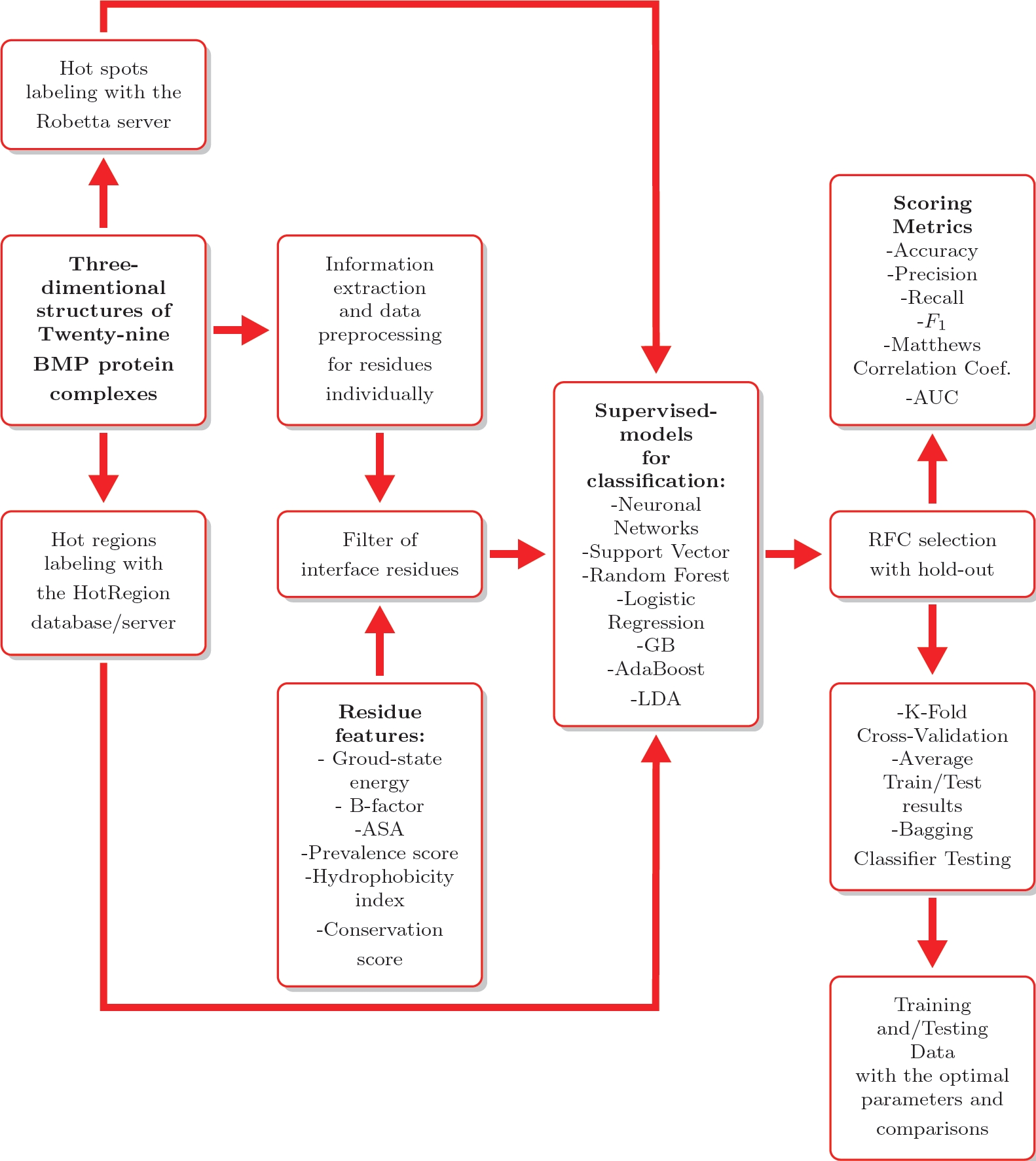
Fig. 2 General training, preprocessing and evaluation processes based on supervised machine learning
Comparing several machine learning techniques, we trained a neural network (multilayer perceptron model) with five layers,
Also, we trained a support vector classifier with a radial basis function (rbf):
A hyperparameter-grid search optimization was performed over the parameters of these models using Scikit-learn in the training data.
This optimization was performed in the following classification algorithms: Gradient Boosting (GB), with
Besides, an RFC was trained with different parameters and configurations, such as a bagging ensemble estimator [5]. Regarding the whole dataset, we split it randomly (hold-out technique with ten-folds), where 70% and 30% of this dataset were for training and testing, respectively.
3 Results and Discussion
3.1 Accelerated Performance
We implemented CPU/GPU hardware acceleration techniques during the preprocessing as parallel programming to speed up the ASA and DFT calculations.
Our parallel ASA implementation improves the performance in execution time in contrast with the scalar Python Pdbremix API [31] implementation based on the number of points used to represent the Van der Waals atomic spheres (Shrake & Rupley approximation).
In the ASA calculation case, the parallel GPU implementation gets a speed-up ratio between three to twenty-two times, reducing the execution time as the protein chains become larger in relation to the number of atoms.
These were possible by locally distributing a load of data in each available core using a three-dimensional spatial box, calculating the ASA between the adjacent atoms and residues inside these boxes [7].
This implementation is still not as fast as some applications, such as FreeSasa [24]. However, adapting ASA calculation algorithms such as the Linear Combinations of Pairwise Overlaps (LCPO), using these schemes presented, enables scalability on the calculations according to the protein size.
On the other hand, the DFT calculation showed a slight speed improvement of 3.5 to 4 times (according to the number of CPU cores), as reported in [7].
3.2 Models Testing
The classification models were evaluated with the Accuracy, Precision, Recall,
In the same way, we assessed the binary classification with the Receiver Operating Characteristics (ROC) curves and the Area Under The Curve (AUC).
Previously, some machine learning algorithms, such as Support Vector Classifier (SVC) and Neuronal Networks, were tested and assessed, as well as the RFC.
Their respective average AUC values denoted that the better method is the RFC [7]. The results of the GB, AdaBoost, and LDA classifiers are shown in Table 2:
Table 2 Average performance rates of the additional classifiers. The 0 corresponds to the non-hot spot & non-hot region class, and 1 corresponds to the hot spots and hot region class, respectively
| Class | Precision | Recall |
|
| GB classifier | |||
| 0 | 0.86 | 0.9 | 0.89 |
| 1 | 0.78 | 0.7 | 0.75 |
| AdaBoost classifier | |||
| 0 | 0.85 | 0.88 | 0.86 |
| 1 | 0.72 | 0.68 | 0.7 |
| LDA classifier | |||
| 0 | 0.78 | 0.86 | 0.82 |
| 1 | 0.6 | 0.5 | 0.55 |
These classifiers do not reach enough performance in comparison with classifiers based on decision trees as the RFC.
The results report of the NN, the SVM, and the Logistic Regression classifiers is found in [7]. Furthermore, a single RFC obtained an
The feature importance for this classifier from the most to the least important was: ASA (0.31), ground-state energy (0.18), conservation score (0.16), B-factor (0.12), hydrophobicity index (0.11), and prevalence score (0.09) of feature importance respectively.
3.3 Bagging Random Forest Classifier Test
RFC can be assembled into a bootstrap aggregating ensemble (decision trees), especially when it is necessary to obtain variance reduction [5].
Fig. 3 shows the comparative performance between a single RFC and a Bagging RFC ensemble in the function of the training data percentage, where one hundred percent of the training set represents seventy percent of the total data assigned randomly.
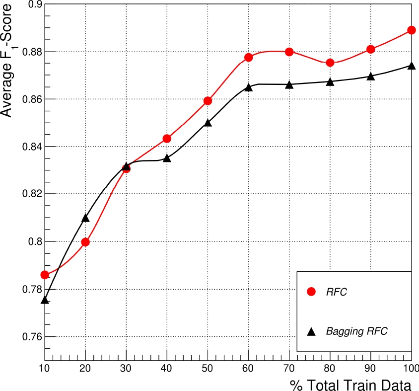
Fig. 3 Average Micro
These experiments show the bagging classifiers based on RFC estimators are less efficient than the single RFC, particularly when the total amount of training data available is used (the 100 percent obtained in both techniques is the best result).
This indicates that many estimators based on trees are over-trained with a loss of generalization for this particular problem. Then, we suggest applying a single RFC model to have better results.
3.4 RFC Validation
The parameters used in the RFC model were the number of estimators or trees and the depth (maximum of samples per tree in the splinted leaves [4]).
In this particular case, we found that applying more than the minimal number of samples per leaf (one) reduces the accuracy of the prediction.
Therefore, to search for the best parameter values and to see the effect of this variation, we followed the next steps:
Firstly, we measured the average of
Fig. 4 expresses non-significant changes in the general performance (
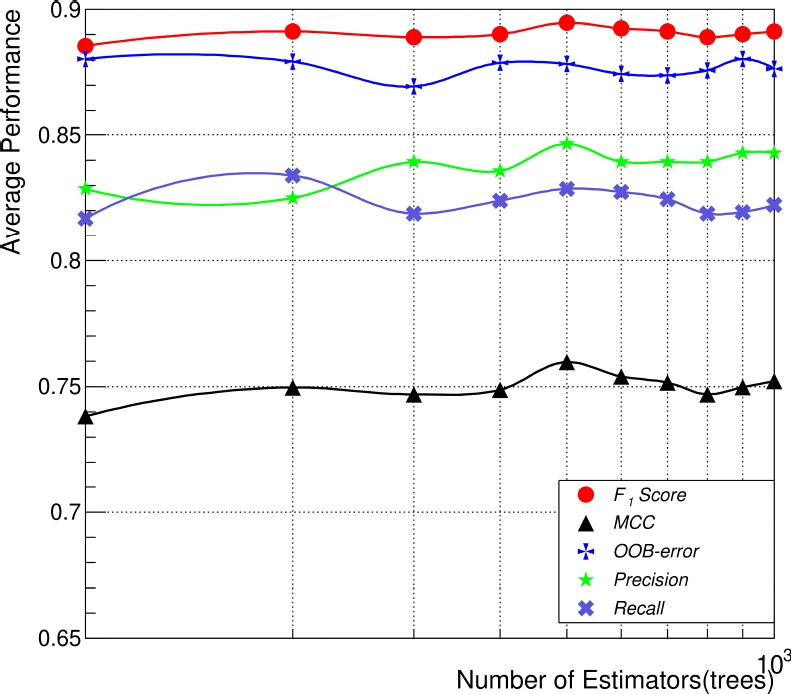
Fig. 4 Average performance comparison between the five performance metrics used, based on the number of estimators or trees in the RFC, in which every point represents a train/test evaluation using 70 and 30, respectively
Secondly, by fixing the number of estimators and varying the depth of the RFC, the metrics reveal a stable behavior after a depth value of 20, reaching an average of
Subsequently, it is possible to set a depth value of 60, from which is obtained a minimal variation (Fig. 5). Using these RFC parameters, the dataset for training and testing was validated with the OOB error varying the total train data as previously.
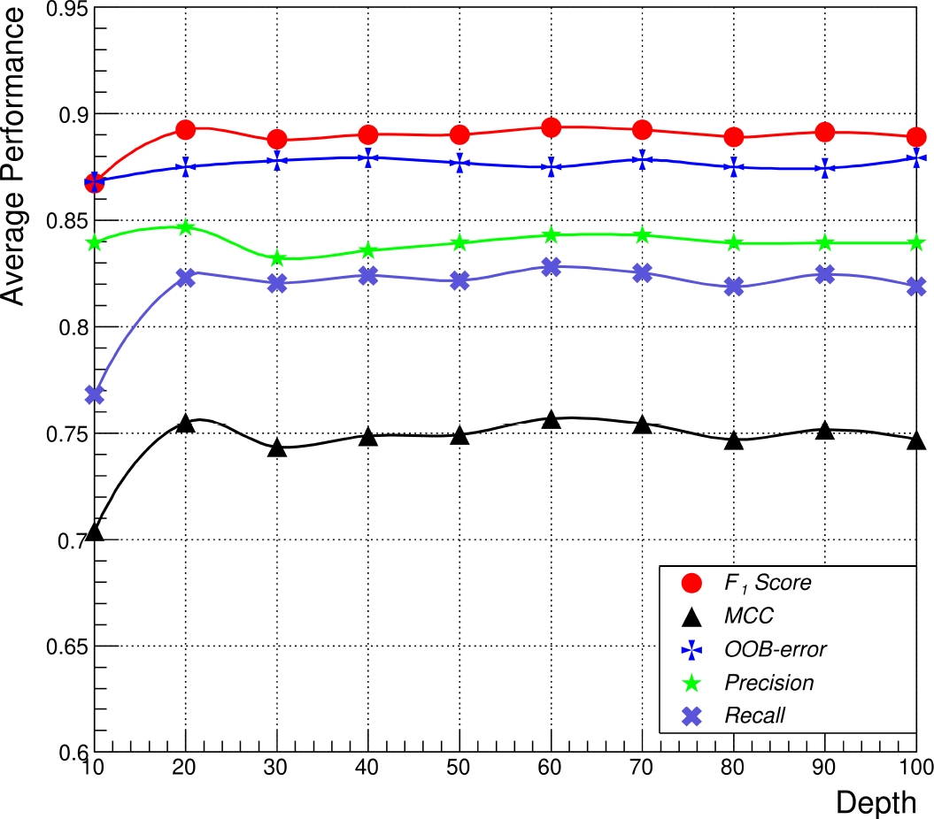
Fig. 5 Comparison of the average performance of the five metrics as a function of the maximum depth of all the trees (fixed as 500 trees) in the RFC, in which every point represents a train/test evaluation using 70 and 30 repeated ten times, respectively
This metric also relates the usage of enough quantity of data for the estimators in the RFC [15]. Therefore, the OOB error reveals an average performance of 0.87, starting at 40% of the training data, showing better stability of the testing output results when we used the training data (see Fig. 6).
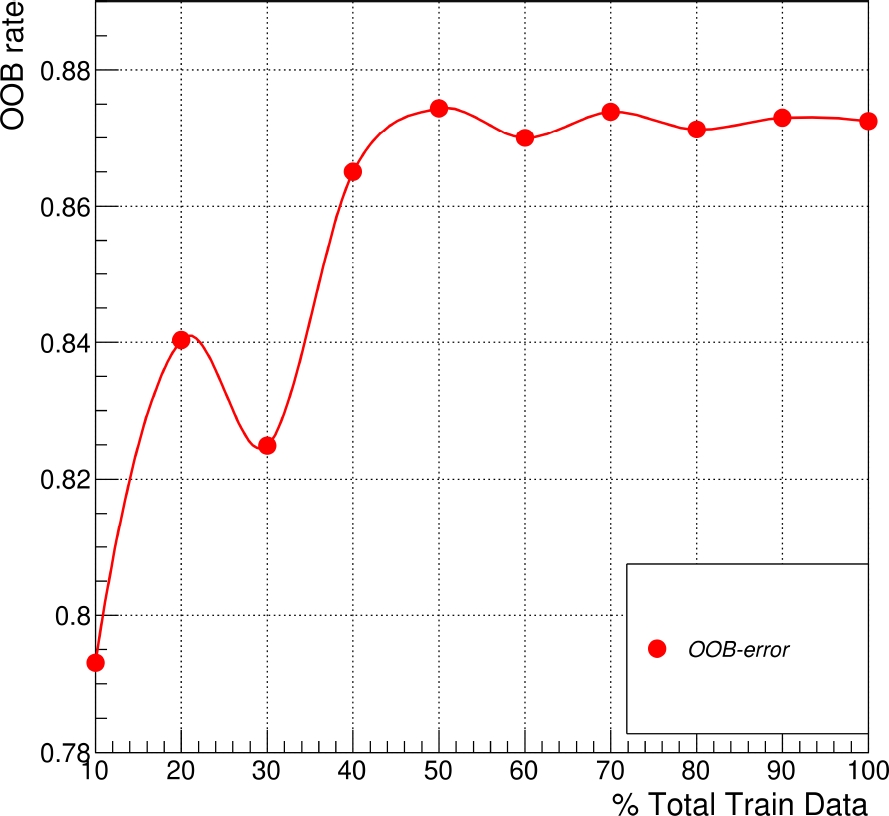
Fig. 6 Average OOB error rates in function of different percentages of data used for training for an RFC with 500 trees and a depth value of 60
Thirdly, the K-fold cross-validation showed the average data consistency between the training and testing proofs. It was applied ten splits repeated ten times (one hundred in total) throughout the whole dataset, obtaining an interpolated ROC curve with an AUC metric of 0.94, which expresses a correlation with low variation.
According to the previous results, the ASA and the ground-state energy areas of the hyperplane of the two-dimensional projection are shown in [7]. This projection supports that the ground-state energy improves the classification.
Besides, training an RFC without the ground-state energy feature obtains an
Table 3 Average performance rates of the RFC. The mean of the accuracy or micro-
| Class | Precision | |
| 0 | 0.92 | 0.0017 |
| 1 | 0.82 | 0.0035 |
| Class | Recall | |
| 0 | 0.91 | 0.0019 |
| 1 | 0.84 | 0.004 |
| Class |
|
|
| 0 | 0.92 | 0.0013 |
| 1 | 0.83 | 0.003 |
Likewise, the average values of (
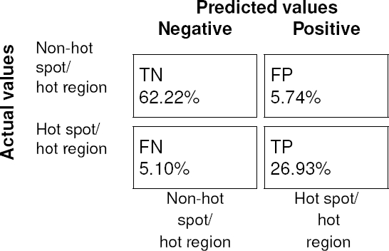
Fig. 7 Confusion matrix of the average RFC. Combining both the true negative (
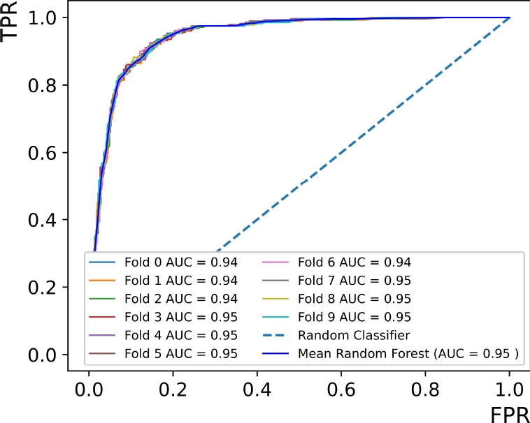
Fig. 8 Average ROC curve performance of ten train/test evaluations. A
We should emphasize that the conservation score is kept as the third and the B-factor as the fourth in feature importance in the whole training process, indicating that these features contribute to the total estimation function of the classifiers also.
The training and testing process using the balanced data does not improve the performance since the
Since almost 70% are not hot spot & hot regions class, the balance data lost relevant information. An advantage of this model is that the RFC training time is faster than the others.
Conversely, the execution time of the DFT algorithm is the main disadvantage of this method. This problem is treated by applying High-performance computing (HPC) or hardware acceleration techniques using deeper parallel implementations.
In addition, DFT can reveal the relation between the electronic configuration energy in the ground state and the binding free energy of the amino acids.
Moreover, we compared the label test data with the foldX ASM framework [10] (for each complex protein in the test data), in which we got
The method for labeling hot spots (ASM from Robetta) has a similar principle [16]. However, the high deviation corresponds to the addition of hot regions (which foldX ASM does not estimate), so a direct comparison is not allowed in this particular case.
Consequently, the RF comparison with foldX test data was
4 Conclusion and Future Work
The RFC proved to be a suitable method for predicting and detecting hot spots and hot regions using this fetched dataset.
A single RFC brings the best results over the rest of the machine learning models applied with this set of features and configurations, including the Bagging RFC classifier ensemble.
Notable advantages of this method are its non-linearity capability separation and the easy and light implementation according to the metrics used in this work.
The main limitation of this work was the completion of the dataset, which needs the DFT calculation in interface residues.
In this sense, DFT calculation is still a hard computational chemistry challenge, which needs several computational strategies to reduce the execution calculation time.
Consequently, the development of acceleration techniques in software and hardware for calculating protein parameters and model refinement is crucial because of the constant increase of data and the current higher computational resources demanded.
A strong result of this work is that the ground-state energy was the second most relevant feature scored, used by the RFC to classify hot spots & hot regions.
This highlight that this feature reveals important energetic information about the protein-protein interactions of BMPs and could help to clear up biological activity. Therefore, expanding the dataset to continue extracting information (especially adding the ground-state energy) should be reinforced.
Consequently, we explored the parallelization via GPU of the ASA calculation (Shrake and Rupley approximation), improving the execution time in contrast with the scalar process. However, the parallelization of newer ASA calculation algorithms should be adapted to obtain better performance.
Finally, a single RFC trained with the six features mentioned above can describe hot spots and hot regions at the protein-protein interfaces with optimal parameter selection with enough performance described by the classification metrics.

