


 text new page (beta)
 English (pdf)
 Article in xml format
 Article references
 Send this article by e-mail
 Cited by SciELO
  Similars in
SciELO
Similars in
SciELO 
 Permalink
1 Introduction
One of the advantages that make decision trees one of the most effective techniques when faced with a problem of supervised learning is the ease of interpreting the predictions made [9]. However, the use of a single decision tree means that the model found has little capacity for generalization, which is known in the literature as overfitting the training data. The use of ensemble methods can be used to face this problem. An ensemble of decision trees is known as decision forest.
This type of model seeks to combine the predictive power of many different decision trees [11]. An important parameter to build a decision forest is the size of the ensemble. This parameter often depends of the data used, however, 100 decision trees is often taken as default value [11, 7, 10].
Because of this, in many cases, more trees are used than necessary, which is expensive in terms of computational resources (memory and processing time).
Hence it its important to detect when adding new trees will not result in an increase in the accuracy of the ensemble, to stop building the ensemble. Different approaches have been proposed to try to solve this problem:
– The method proposed in [10] consists of estimating the number of classifiers that are necessary to reach a prediction that, on average, coincides with a hypothetical ensemble of infinite size with high probability as infinity approaches 1. In contrast to previous proposals found in the literature this procedure is not based on estimating the generalization error.
– In [1] the authors compare a variant of the randomized C4.5 method, random subspaces, random forests, AdaBoost.M1W, and bagging. This is the largest comparison of ensemble techniques that we are aware of, in terms of number of data sets and number of techniques. The authors also showed a way to automatically determine the size of the ensemble. The stopping criteria they presented showed that it is possible to intelligently stop adding classifiers to an ensemble using the out-of-bag error.
In this paper, a new method is proposed to reduce the amount of trees to be built in a decision forest, maintaining the accuracy of the classification.
The idea is to incrementally add decision trees until a stopping criterion based on the accuracy is used. The proposed method is incorporated to the Proactive Forest and Random Forest algorithms, to detect when to stop the construction of the decision forest while maintaining the accuracy.
In addition, the proposed method is compared against the method proposed in [1].
2 Methods to Determine Ensemble Size
The use of ensembles in classification tasks has been proposed by numerous authors in the machine learning literature [7, 2, 3, 17, 16, 12, 15].
These studies show that combining the decisions of complementary classifiers is an effective mechanism to improve the generalization performance of a single predictor.
The ensemble methods construct and combine multiple models to solve a particular learning task. This methodology imitates the nature of human beings to seek several opinions before making a crucial decision such as choosing a particular medical treatment [3].
The fundamental principle is to give a weight to each of the individual opinions and combine them all with the objective of obtaining a decision that is better than those obtained by each one of them separately [12, 16].
It has been shown repeatedly that ensemble methods improve the predictive power of an individual model [11]. These methods work particularly well when they are used with decision trees as base models.
This combination is what gives rise to the term decision forest [16, 17]. One of the most important elements when building a decision forest is the number of trees that will be used.
There is no consensus regarding the size that a forest must have to obtain the maximum possible accuracy value in classification. In the last years different solutions have been developed for this problem, each one tries to solve it from different approaches and construction schemes.
Among them the most important are: The method proposed in [1] suggests that using an appropriate ensemble size is important. They introduce an algorithm that decides when a sufficient number of classifiers has been created for an ensemble.
This algorithm uses the out-of-bag error estimate, and it is shown to result in an accurate ensemble for those methods that incorporate bagging into the construction of the ensemble. This work estimates the accuracy using the out-of-bag prediction.
Episodes are built composed of twenty classifiers for each one, the efficacy is calculated by subsequently applying a technique of smoothing the accuracy as follows; average accuracy is calculated for each of the twenty classifiers, for the first classifier, the smoothed accuracy will be its own.
For the second it is the average between the first and the second. So up to five, which would be the average from the first to the fifth. Now for the sixth it would be from the second to the sixth, since the size of the smoothed accuracy is five.
So until completing the twenty classifiers that make up an episode. The maximum smoothed accuracy value for the episode is then saved.
The necessary episodes are constructed in the same way. The construction stops when comparing the smoothed value of an episode with that of the previous one, it is less than or equal.
In [10] the authors take advantage of the convergence properties of majority voting to determine the appropriate size of parallel ensembles composed of classifiers of the same kind. The statistical description of the evolution of the class prediction by majority voting in these types of ensembles has been extensively analyzed in the literature.
This method [10] differs from the previous proposals that are based on stopping the construction of the ensemble when accuracy is stabilized. It is based on the statistical description of the convergence of the majority voting to its asymptotic limit and assumes that a parallel ensemble and majority vote is used.
For each instance, the minimum size of the ensemble is determined, for which, it will not change its labeled class when adding more models. Then, a consensus is reached between the size indicated by each instance and that is the final size.
In [12] the authors offer a way to quantify this convergence in terms of algorithmic variance, i.e., the variance of prediction error due only to the randomized training algorithm.
Specifically, they study a theoretical upper bound on this variance, and show that it is sharp in the sense that it is attained by a specific family of randomized classifiers.
The proposed method is inspired by Progressive Sampling [14]. In Progressive Sampling the objective is to find an optimal sample of the data that can be used to classify, without using the entire data set [8].
To do this, an analysis of the accuracy generated by different samples of the data is made, as the samples are analyzed, their size is increased.
Based on this idea, a study of the behavior of classification accuracy was carried out using a proactive decision forest construction algorithm proposed in [4].
In this case, a tree was incrementally added and the accuracy of the random forest was evaluated until reaching 100 trees.
This study allowed us to understand how the accuracy of the databases behaved and clearly illustrates that some classification problems can be solved with few trees and that incorporating more trees does not improve the accuracy.
3 Results: Progressive Forest
The Progressive Forest method builds the forest considering episodes of 5 trees as parameter, each time a new tree is added to the forest the accuracy of the ensemble is calculated up to that model and the maximum and minimum values of accuracy of the episode are extracted.
To establish how many trees should make up an episode, several tests were carried out, showing that 5 trees is an appropriate size, taking into account that the maximum number of trees to be created in the forest is 100 and trying to stop the construction of the ensemble as soon as possible.
This process is repeated until finding a point where the maximum value minus the minimum value is less than or equal to parameter 0.002 during two consecutive episodes. This value was experimentally validated, and it is used to determine convergence.
When this condition happens, it is assumed that accuracy has entered into a convergence process and that adding new trees will not translate into better accuracy. Later the ensemble is truncated, at the maximum accuracy point of the last episode.
The pseudocode of the Progressive Forest method is shown in Algorithm 1. In step 1 of the algorithm pseudocode, the convergence value used was 0.002.
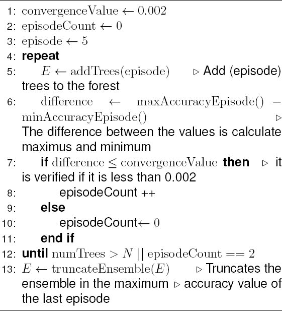
To define this value, an empirical study was carried out in which the mean, mode and median of each of the episodes were analyzed and it was decided to establish 0.002 as the convergence parameter.
When the subtraction of the maximum and minimum of the precision of an episode is equal to or less than this value, the accuracy is converging to a plateau. Furthermore, it was decided that this should be true for two consecutive episodes to ensure convergence before stopping the algorithm.
In step 3, the size of the episode is defined as size 5. To establish this value, an empirical study was also carried out, which allowed establishing two basic characteristics for the construction of the episodes: first, the need to make an episode to achieve a better understanding of the behavior of the efficiency, since analyzing it individually did not allow defining a convergence point.
Secondly, it should be a small value because the objective of the algorithm is to stop the construction of the forest early, without affecting the classification efficiency.
Experiments were carried out with different values, which allowed deciding that the best size was 5, since it is relatively small and allows analyzing the convergence of the efficiency.
Further studies can perform a deeper analysis of these parameters and perhaps improve the results of the algorithm.
4 Experimentation
In this section it is described how the experiments were performed, the main results are presented and analyzed, and the limitations of the proposed method are described.
4.1 Configuration of Experiments
Cross-validation was used to evaluate the accuracy of the proposed solution. In particular, the cross-validation technique of k-iterations (k = 10) was used, where the data are separated into k subsets, one of the sets is used as a test set and the remaining k-1 as training data.
To make the validation process more robust, the results are obtained using a 5 times 10 fold cross-validation process.
This guarantees that the results are independent of the partition between training data and test data. It is used in environments where the main objective is prediction and we want to estimate how accurate the model is.
For the realization of the experiments, datasets of diverse characteristics get from the UCI Machine Learning repository were used [6].
The dataset contain from 3 to 64 attributes, from 2 to 26 classes, and from 106 to 20000 instances. Only one dataset has missing values, however, 22 of the 31 datasets have class imbalance. The Table 1 shows the description of the datasets used.
Table 1 Dataset description
| Dataset | Instances | Attributes | Imbal. |
| Balance scale | 625 | 4 | x |
| Car | 1798 | 6 | x |
| Cmc | 1473 | 9 | x |
| credit-g | 1000 | 20 | x |
| Diabetes | 768 | 8 | x |
| Ecoli | 336 | 7 | x |
| flagsreligion | 194 | 29 | x |
| Glass | 214 | 9 | x |
| Haberman | 306 | 3 | x |
| heart-statlog | 270 | 13 | |
| Ionosphere | 351 | 34 | x |
| Iris | 150 | 4 | |
| kr-vs-kp | 3196 | 36 | |
| Letter | 20000 | 16 | |
| Liver | 345 | 6 | |
| Wine | 178 | 13 | |
| Lymph | 148 | 18 | x |
| Molecular | 106 | 58 | |
| Nursery | 12960 | 8 | x |
| Optdigits | 5620 | 64 | |
| page blocks | 5473 | 10 | x |
| Pendigits | 10992 | 16 | |
| Segment | 2310 | 19 | |
| solar flare 1 | 323 | 12 | x |
| solar flare 2 | 1066 | 12 | x |
| Sonar | 208 | 60 | |
| Spambase | 4601 | 57 | x |
| Tae | 151 | 5 | |
| Vehicle | 846 | 18 | |
| Vowel | 990 | 13 | |
| Wdbc | 569 | 30 | x |
For the analysis of the results obtained, the Friedman statistical test was used to know the algorithm that generates the highest accuracy value, the number of trees built, and the construction time [13, 5].
Additionally, the post-hoc Holm, Finner and Li [13] are applied to determine if there are significant differences between the algorithm with the best ranking in the Friedman test and the others.
To run the statistical tests, a significance level of
To validate the solution presented, the Proactive Forest (PF) and Random Forest (RF) algorithms are used, in their original construction schemes, with the method proposed in Banfield [1] (PF BAN and RF BAN, respectively), and with the method proposed in this article (PF MM and RF MM, respectively).
Table 2 shows the results obtained with the Friedman test for the Proactive Forest algorithm. From Table 2 we can observe the following:
Table 2 Ranking obtained using the Proactive Forest algorithm
| Accuracy | ||
| No. | Algorithm | Ranking |
| 1 | PF | 1.58 |
| 2 | PF MM | 2.13 |
| 3 | PF BAM | 2.29 |
| Number of Trees | ||
| No. | Algorithm | Ranking |
| 1 | PF MM | 1.37 |
| 2 | PF BAM | 1.65 |
| 3 | PF | 2.98 |
| Time | ||
| No. | Algorithm | Ranking |
| 1 | PF BAM | 1.29 |
| 2 | PF MM | 1.71 |
| 3 | PF | 3.00 |
– Proactive Forest in its original scheme has the best accuracy values with a significant difference between PF and both PF MM and PF BAN.
– In terms of the number of trees, the proposed method (PF MM) has the best ranking, there is a significant difference between PF MM and PF and between PF BAN and PF, but not between the PF BAN and the PF MM.
– Regarding time, PF BAN has the best ranking followed by PF MM, with a significant difference between the PF MM and PF, but not between PF MM and PF BAN.
Figure 1 shows the average obtained by the Proactive Forest algorithm with the objective of better visualizing the results presented above. Table 3 shows the comparison of the average behavior of the algorithms for all data set.

Table 3 Comparison of the average behavior of the algorithms using Proactive Forest
| Accuracy | |
| PF MM vs PF | PF BAM vs PF |
| 99.65% | 99.47% |
| Number of Trees | |
| PF MM vs PF | PF BAM vs PF |
| 55.14% | 60.27% |
| Time | |
| PF MM vs PF | PF BAM vs PF |
| 63.80% | 57.40% |
As shown in Table 3, the proposed method has a very similar accuracy to the original method (99.65%), but with a significant reduction in the number of trees used (55.14%) and in the processing time (63.80%).
It has better accuracy and a lower number of trees than BAN but it uses more processing time. Table 4 shows the results obtained for Random Forest with the Friedman test. As can be seen from Table 4:
– Random Forest, in its original scheme, is the best ranked in terms of accuracy, followed by RF MM, with a significant difference between RF and both RF MM and RF BAN.
– Regarding the number of trees, again RF has the best ranking followed by RF BAN. There is a significant difference between RF MM and RF BAN with regard to RF, but not between the RF BAN and the RF MM.
– Regarding time, in this case the best ranked method is RF MM followed by PF BAN, and there is a significant difference between RF MM and both RF and RF BAN.
Table 4 Ranking obtained using the Random Forest algorithm
| Accuracy | |
| PF MM vs PF | PF BAM vs PF |
| 99.65% | 99.47% |
| Number of Trees | |
| PF MM vs PF | PF BAM vs PF |
| 55.14% | 60.27% |
| Time | |
| PF MM vs PF | PF BAM vs PF |
| 63.80% | 57.40% |
Figure 2 shows the average obtained by the Random Forest algorithm with the objective of better visualizing the results presented above. Table 5 shows the comparison of the average behavior of the algorithms in all the data sets.
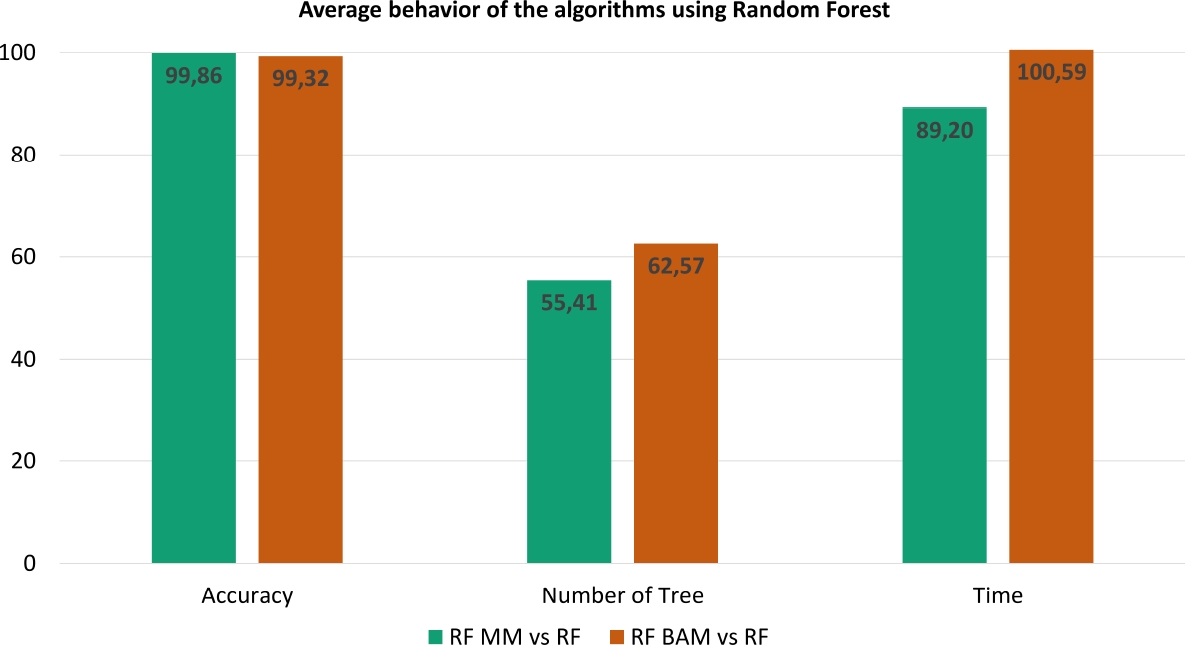
Table 5 Comparison of the average behavior of the algorithms using Random Forest
| Accuracy | |
| RF MM vs RF | RF BAM vs RF |
| 99.86% | 99.32% |
| Number of Trees | |
| RF MM vs RF | RF BAM vs RF |
| 57.41% | 62.57% |
| Time | |
| RF MM vs RF | RF BAM vs RF |
| 89.20% | 100.59% |
From Table 5 it is shown that the proposal presented maintains a very similar classification accuracy as the original Random Forest algorithm (99.86%), with a significant reduction in the number of trees used (57.41%) and with less processing time (89.20%).
In this case, the algorithm shows very competitive performance with respect the method proposed in [1].
4.2 Discussion
Below are some significant elements extracted from the analysis of the experiments:
– Progressive Sampling is an effective method to build smaller ensembles with less processing time and with competitive accuracy when compared to the original algorithms.
It proves experimentally that, for some datasets, there is no need to add more models to improve the accuracy.
– When Progressive Forest is compared to [1], in general, it has better accuracy and uses less trees but has mixed results in terms of processing time.
This can be easily explained in terms of how many trees are used to evaluate the ensemble. In the proposed method, we propose to evaluate every 5 models while Banfield [1] evaluates every 20 models.
In some cases, using 20 models, means that at least 40 models will be needed to decide when to stop the construction process, when a much smaller of models may be needed.
On the other hand, evaluating every 5 models means that our proposed method will make , in some cases, more evaluations than [1].
4.3 Limitations
Progressive Forest, in classification problems with very few instances, does not always work as expected, since partitions with very few data produces inaccurate results.
The proposed method measures the difference between the maximum and minimum for each episode and only this difference is taken into account to stop the construction process.
In some cases, there are still differences in these values and the construction process could be continued with more than 100 models, with 200 and even 2000, but this in general does not improve accuracy as shown in [10].
Another reason why one does not look if the current episode is greater than the previous one is because of the reliability of the test set, even in [1] where they compare to see if the maximum accuracy value stops increasing they use smoothing techniques and do not take the raw accuracy points.
5 Conclusions and Future Work
In this paper, a new method, called Progressive Forest, to stop the construction of a decision forest is presented.
This proposal can be incorporated into any ensemble construction scheme similar to Random Forest type. Progressive Forest was incorporated into the construction schemes of Proactive Forest and Random Forest, and compared with a method proposed by Banfield.
From the experimental results, it is shown that in comparison with the original ensembles methods, a smaller number of models can be used, with a reduced processing time, while maintaining the accuracy of the classification.
There are several research areas that could be explored as future work. First, analyze in greater depth the dependence of the estimation of accuracy with respect to the size of the ensemble.
Second to carry out a study of correlation between the effort generated by the addition of new models and the accuracy that would be gained. Third, carry out a study of the characteristics of the data set to identify in what types of problems the proposed solution is most effective.
Fourth, carry out a systematic study of the parameters defined in the proposed method and their effect in its performance.Fifth, determine which variables can be taken into account to control the stopping of the decision forest.

