


 text new page (beta)
 English (pdf)
 Article in xml format
 Article references
 Send this article by e-mail
 Cited by SciELO
  Similars in
SciELO
Similars in
SciELO 
 Permalink
1 Introduction
1.1 General Background
Segmentation of clusters of overlapping or touching objects in binary images into their single components has been addressed in a variety of practical situations and continues being an open research topic in Image Processing.
Examples can be found for the case of two-dimensional gel electrophoresis overlapping spots [36], segmentation of rocks in images with application to mining industry [4] and rock particles in general for their recognition [39].
Other examples are applications related to nanotechnology [43] and to agriculture and food [3], general automated size analysis in multi-flash imaging [21] as well as numerous applications in the biomedical field, among which segmentation of overlapped or touching erythrocytes in microscopy images, to which this work is devoted, is an important example.
A classification of the segmentation methods used in a specific biomedical application is presented in [19] where various approaches like methods based in concave point detection, blob detection, clustering and morphological processing are recognized and discussed.
Other examples are splitting of clumped or overlapped cells based on template matching strategy [7] and a method called Recursive Water Flow (RWF) [8] for cell splitting in histological images. The problem of segmenting touching cells in a 3D framework is addressed in [23].
Segmentation of histopathological images including overlapped or touching cells was addressed in [13] using deep learning algorithms and spatial relationships. Splitting of 3D cell clusters for the case of volumetric confocal images is presented in [15].
A combined method for overlapped cell detection and segmentation based in features obtained from the skeleton and the contour of the cells is showed in [16]. A semi-automatic approach for detection and segmentation of cell nuclei based on graph-cuts and Laplacian of Gaussian (LoG) filtering is proposed in [1].
A method based on concave points extraction through polygonal approximation and ellipse fitting bubbles with average distance deviation criterion and two constraint conditions was addressed in [45]. Reference [44] employed a modified version of curvature scale space method to extract corner points and then recognize the concave points by evaluating angular changes.
These concave points and the centroid points are then used to characterize the structure of the cell clump and to construct the split line by using the corresponding splitting strategy. Other approach proposed recently to split overlapped cells based on elliptical shape models appers in [29].
Various approaches to segment clusters in images from the Papanicolaou test are presented in [31, 32, 33, 38] and other diverse microscopy image applications using methods not based in mathematical morphology were reported in [28, 27, 34, 41].
The method proposed in this work uses an approach to segment clusters based in morphological image processing techniques and under such view, we will comment about methods of this kind in more detail. A method to split cell clumps based in the use of different morphological scales after iterative erosion to find cell-specific markers is developed in [37].
In spite of the good results they obtained, the authors point out that at the time of their publication a comprehensive benchmark using a database of cell clumps or clumped objects was not available. It is worth to notice, however, that to our knowledge such benchmark does not exist yet.
A morphological method is presented in [17] based in the use of an adaptive H-minima transform together with an external distance and marker-controlled watershed transform to segment cell clusters, with good results in terms of percentages of correctly segmented clusters.
Reference [18] followed this line of work and it was introduced there a parameterization using an ellipsoidal modeling of contours to perform a more appropriate analysis. The authors expressed their results there in terms of percentages of correctly split clumps.
Various alternatives of the use of markers considering minima imposition were studied in [6] where a relative equivalence was found between different approaches, to represent the markers used to control the watershed transform in order to split the clumps.
Other morphological approach using the watershed transform complemented with a corner detection algorithm appears in [26]. The classical watershed and distance transforms are used in [40], specifically to segment chromosomes showing overlapping.
An improved ultimate erosion process (UECS) together with an edge-to-marker association is proposed in [30] to separate the overlapping convex objects in electron micrographs.
In this work, the authors used a noise-robust measure of convexity (or concavity) based on the sensitivity to the coarseness of digital grids as the stopping criterion for erosion. The missing contours of the occluded particles are inferred using a Gaussian mixture model on B-splines.
In reference [42] the gradient-barrier watershed algorithm is proposed, in which the gradient in the overlapping region is used directly as the barrier to the water flow. A cluster segmentation method based in the use of structural features and morphological image processing is showed in [20], again obtaining high accuracy in terms of performance measures (sensitivity, specificity) of the cluster detection process as well as accuracy of segmentation.
A review of the use of mathematical morphology techniques in malaria studies, which includes the segmentation of overlapped cells is presented in [25]. Reference [22] presents a method based in a watershed algorithm that iteratively identifies markers, considering a set of different h values in the H-minima transform.
This method showed good results, but it is oriented to the specific case of wide-field fluorescence microscopy images and requires calculating a fair gradient map from the original image as well as defining heuristically some parameters.
Recently, deep learning algorithms, in particular convolutional neural networks (CNN) have been also applied in medical image analysis [24]. The fully convolutional neural network U-Net [35] has significantly influenced the field of cell segmentation.
This network model was designed to work with few training images and to obtain accurate segmentation. In [2] deep learning was applied to predict cell nuclei and combined with thresholding and watershed transform to segment different types of cells.
Their approach was developed only for fluorescent images with stained cytoplasm. A modified version of U-Net called MultiResUnet is proposed in [14] and obtained better results than using the classical U-Net.
In reference [12] is proposed a method called BubCNN which employs a Faster region-based CNN (RCNN) detector module to locate bubbles and a shape regression CNN to predict bubble shape parameters.
A great future can be foreseen for deep learning based models in this kind of applications, however training deep networks tends to be computationally expensive and might require large numbers of annotated data, which is a time-consuming process. This implies that other conventional image processing techniques like those presented here can be still a valuable choice for the task addressed in this work.
1.2 Unified Framework for Detection and Segmentation of Clusters
We introduce in this work a unified method oriented to segment with high effectiveness clusters having up to medium complexity, which means roughly less than 30% overlapping which could be considered to allow a useful individual cell analysis after splitting. We mention also that erythrocytes consist usually in round-like objects of moderately variable sizes.
The algorithm used to segment the clusters operates by means of a combination of the conventional distance transform, the H-maxima transform, morphological operations and a weighted external distance transform combined with marker-controlled watershed segmentation, as will be described in detail later. This allowed using the information obtained during the clusters detection to facilitate their subsequent segmentation (split).
The method presented here showed a high effectiveness in detecting the clusters in terms of performance measures like sensitivity, specificity, accuracy, precision and F-measure, as well as a high segmentation accuracy. The latter was measured in terms of the Jaccard index obtained when comparing the computer-segmented objects to a manually segmented ground truth.
2 Materials and Methods
2.1 Images Dataset
The whole detection and segmentation process begins with a coarse segmentation, which produces a binary image in which the touching or overlapping erythrocytes remain as connected components. The binary images used in our experiments contain clusters of various sizes and were obtained through coarse segmentation of microscopy images, which correspond to mice peripheral blood smears stained with Giemsa.
Other components of the blood smears as leukocytes and platelets were eliminated from the image using image processing techniques, not described here as our interest resides in the segmentation of the remaining clusters of erythrocytes.
A Zuzi microscope model 148 was used to acquire the images, equipped with a plan-achromatic lens having 1.25 numerical aperture and a 0.5 magnification of the camera adaptor, with a 319CU digital camera of 3.2 megapixel and 8-bit RGB uncompressed output, obtaining a resolution of 2048 × 1536 pixels. The objective power used was 100× with immersion oil, obtaining a total magnification of 50×, which results roughly in around 140 pixels per cell diameter for the images employed in the experimental work.
The images were saved in.tiff (tagged image file) format. Then, the images were segmented by thresholding to obtain the set of binary image containing independent, single objects as well as clusters of various sizes and complexity.
Other steps in this process included conversion to grayscale prior to thresholding and then, morphological area-opening filters are used to remove items smaller than a red blood cell and to fill the holes left after thresholding. We stress the fact that this primary ”coarse” segmentation is not of concern to this research and its role was only to obtain images containing appropriate clusters to perform the experimental work.
The dataset created consists of 43 images containing in total 4265 binary objects, 1081 of which can be considered as clusters and 3184 as individual cells. Fig. 1 shows an original image and its corresponding binary image after coarse segmentation and Fig. 2 exhibits four examples of connected regions forming clusters.

Fig. 1 Microscopy image and coarse segmentation (a) original image (b) coarse segmentation from image (a)

2.2 Detection of the Clusters Contained in the Binary Images
To detect the clusters contained in the binary images that were obtained as described in the previous section, we followed a method that uses both the conventional (inner) distance transform, the external distance transform (EDT ) and a weighted version of it (WEDT ) as well as the H-maxima transform and some morphological processing operations, in a process described in detail in what follows.
This approach was used because it produces the inner markers needed afterward in the splitting process. The distance transform
To calculate
As the inner distance transform is applied here to the complement of a connected component, its result is a grayscale image exhibiting its highest intensity in a point or patch, which is in general a regional maximum, located farthest from the background. This process is depicted in Fig. 3.
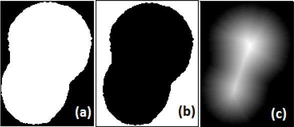
Fig. 3 (a) Binary image from overlapping cells. (b) Complemented binary image. (c) Distance transform
The eventual appearance of spurious maxima will be addressed later. To define the external distance transform, consider the set
Then for any point
The proposed methodology followed a sequence of steps to determine whether a connected component in the binary image (obtained from the previous coarse segmentation) corresponds to a cluster or to a single object and then, split those that are considered as clusters. These steps were:
Labelling the connected components and calculating the inner distance transform map for each one.
Obtaining the valid regional maxima of the distance transform (DT ) for each binary object present in the image).
Classify as clusters all the objects having more than one of these maxima.
Build the skeleton by influence zones (SKIZ) [9] which correspond to the regional maxima for each cluster, using the weighted EDT (WEDT ), which is the EDT with its values divided (weighted) by a factor obtained during the selection of the valid regional maxima described in the next section.
Segment the clusters into their constituent components by means of the marker controlled watershed transform [9], using the SKIZ lines as external markers and the regional maxima as inner markers.
When building the EDT map in setp 4 to obtain the SKIZ, the distances from a background pixel to each regional maximum were weighted by a coefficient, which depends on the magnitude (height) of the regional maximum, previously normalized to the interval [0, 1]. Segmentation by means of the watershed transform followed the previous steps.
We point out, however, that obtaining valid regional maxima corresponding to the clustered binary objects is not a trivial task. The clusters may have a moderately irregular contour, and therefore several spurious maxima can appear after calculating the distance transform.
These spurious maxima are usually deemed as noise and can lead to over segmentation when used as markers for segmenting using the marker-controlled watershed transform.
2.3 Determining the Valid Regional Maxima in DT(A)(x)
In this work, three methods were applied and compared in order to determine the valid regional maxima present in the binarized clusters.
— Method 1: Iterative H-maxima transform. This method apply iteratively the H-maxima transform to the distance transform map of each complemented binary objects and afterwards counting the number of remaining regional maxima.
— Method 2: Morphological filtering. This method has the purpose of transforming the set of spurious regional maxima formed around the center of a single (and perhaps part of a cluster) object into one valid, unique maximum.
In this case, an alternating open-close sequential filter [9] with two stages and a disk structuring element is applied to the distance transform map. Then, the algorithm extracts the regional maxima and the magnitude (height) of these resulting maxima is considered representative of that of the individual merged maxima.
— Method 3: Radon transform. This method is described in [11] where the Radon transform and morphological operations are used to find the markers for the erythrocytes.
A detailed description of these methods is presented in the next section.
2.4 Detailed Description of the Methods Used to Detect Clusters
The H-minima and H-maxima transforms are powerful tools to suppress undesired minima or maxima in a grayscale image.
In this case, we applied the H-maxima transform to the distance transform map corresponding to the complemented binary image, obtained from the coarse segmentation step. The H-maxima transform HMAX is defined in [9] as:
where
This fact is used in as stop criterion in [17], where the dual H-minima transform is used in an analogous way. The algorithm in this reference goes back one step to keep isolated the regional minima pertaining to different adjacent merged objects.
However, increasing h in small steps until merging the maxima from adjacent objects implies in our case an unnecessary computing burden, because actually there is only the need to suppress the spurious maxima, which will occur after only some few steps.
In order to find a practical solution to this problem, experimental work with a large number of diverse clusters was performed, testing the results of iterations increasing the parameter h.
It was found experimentally that the number of maxima stabilizes in the desired value after at least five successive iterations in practically all cases, without further decrements in the number of maxima until the merging phenomenon previously mentioned occurs.
This determined the use as stop criterion for the iterative H-maxima transform the constancy of the number of detected regional maxima during five successive iterations. If after this convergence more than one maximum remain present in a connected component being analyzed, it is possible to say that we are in presence of a cluster, given that a single erythrocyte would show only one maximum.
Then, the maxima obtained for the different components in the image are saved. These maxima will be used later as internal markers to be used in the watershed segmentation, together with the last height value obtained from the HMAX transform, which will be also used for separating the clusters into individual objects. On the basis of the previous discussion, three methods to detect clusters were implemented and compared, whose algorithms are summarized as follows:
2.4.1 Method 1: Iterative H-maxima Transform for Detecting Clusters
Perform the coarse segmentation of the image using a standard method and label the resulting binary connected components, which can be either single objects or clusters.
-
For each labeled object i do:
a) Compute the distance transform (Euclidean) on the complement of the ith connected component and normalize the obtained grayscale image Dmap to the range [0,1].
b) Count the number of regional maxima in Dmap for each labeled connected component; let this number be N.
c) Guess an initial parameter value
d) While
This was the criterion of convergence for the calculation of the number of maxima and the suppression of spurious extrema. Here in each iteration the new value of N is saved and compared with the previous one, to allow counting the number of repeats of it. Every time N changes, the counter is reset to one and counting re-starts.
e) If
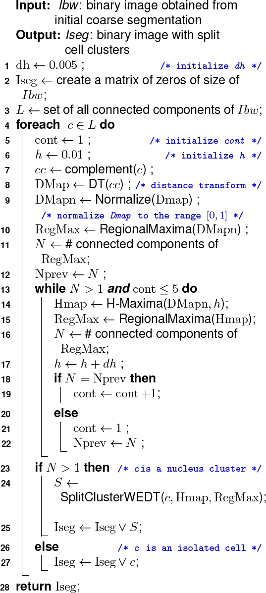
The pseudo code illustrates this algorithm for the Iterative H-maxima transform method. Fig. 4 shows a binary object corresponding to a cluster of 2 erythrocytes and the regional maxima obtained for it during its processing. Notice that in this case

Fig. 4 (a) Regional maxima superimposed to the distance transform map in Fig. 2, notice the presence of multiple spurious maxima. (b) Final regional maxima after the iterative search, where the spurious maxima have been merged into two single ones, as expected
2.4.2 Method 2: Morphological Filtering
This method applies a morphological approach to detect clusters and extracting markers for both the clusters and the single cells. The steps are as follows:
Perform the coarse segmentation of the original image in the same way as in Method 1.
Determine the distance transform (Euclidean) of the complement of this binary image and then normalize it. Let be Idt the resulting image.
Compute a two-stages open-close alternating sequential filtering (ASF), using a disk structuring element g with radius 1 and 2 in the first and second filtering stages respectively, in order to eliminate the spurious maxima. We call the resulting image Ioc. The general expression for this filtering process is:
For which in this case f is the Idt image. Here
4. Determine the regional maxima on Ioc and call the resulting image Irm.
-
5. For each labeled connected component present in the binary image:
a) Compute a logical AND operation between the binary image of the connected component and Irm. We call the resulting image Imark.
b) Count the numbers of regional maxima on Imark with the aid of labeling the connected components contained in it.
c) If the number calculated in (b) is greater than one the object is classified as a cluster and its division is carried out using the SplitClusterWEDT method, which receive as arguments the binary image of the cluster, the regional maxima map of the cluster (Imark) and the distance transform image after the open close filtering (Ioc). In other cases, the object pertaining this connected component is classified as a single erythrocyte.
2.4.3 Method 3: Radon Transform (RT)
This method uses the Radon transform to find the markers for the cells as described in [11]. The search for markers is performed based on the ability of the RT to detect shape parameters and their behavior with circular structures.
The circular structure edge was determined previously in order to apply the direct RT and after that the sinogram projections were filtered using a matched filter having a horseshoe-shaped impulse response. This filter was used to enhance the projections of all circular structures with radius r, which is computed from the median cell area in each image.
Then, an image with peaks close to the circular structures centers is obtained by means of the inverse RT. After this, a threshold is applied which is calculated by means of histogram analysis of the reconstructed grayscale image.
Finally, a morphological closing was performed in order to identify the final markers of each cell. Once the image containing the markers is obtained, we proceed to determine which connected components within the coarse segmentation image can be considered as clusters for their subsequent division by means of the SplitClusterWEDT method.
Similarly, to the previous method, for each connected component of the binary image obtained by means of the coarse segmentation, a logical AND operation of it with the whole markers image is performed to obtain the final markers that correspond to the specific connected component that is being analyzed. The resulting markers are labeled and if their number is greater than one the corresponding object is considered as a cluster.
The SplitClusterWEDT algorithm needs three arguments, which in this case are the binary image of the cluster, the markers corresponding to this cluster and the normalized distance transform of the logical complement of the cluster binary image.
As a final comment concerning the last step in the previous descriptions, e.g. calling the method to split the clusters, we emphasize the fact that aside from the cited SplitClusterWEDT method, splitting by means of the classical marker controlled watershed transform as well as using the EDT were also tested and compared, as described in the following section.
2.5 Segmentation of Clusters Into Their Constituent Objects
The algorithm devoted to segment the connected components identified as clusters into their constituent parts takes three inputs. The first one C is the binary image of the cluster. The second parameter RegMax is the binary image of the valid regional maxima identified during cluster C detection.
The third one Hmap depends upon the clusters detection method employed. The output of this algorithm is the binary image Cseg of the cluster, divided into its constituent components.
The algorithm begins by labeling and counting the connected components of the regional maxima contained in RegMax and setting their values in the variables LRM and Num respectively. Then follows a loop having as many iterations as regional maxima are present in C.
This loop starts initializing a binary matrix S to zero and then setting to one the elements of S whose positions match with the elements labeled i in the LRM matrix. The described loop can be implemented instead through vector operations for the sake of computational efficiency.
Then the algorithm computes an element-wise multiplication (Hadamard product) between matrices S and Hmap to obtain a new matrix called HeightRM, whose values correspond, for Method 1, to those of the h-maxima transform in the region occupied by each regional maximum and are zero in the rest of the matrix. In this case, for methods 2 and 3 the values of the distance transform are used instead of the h-maxima transform values.
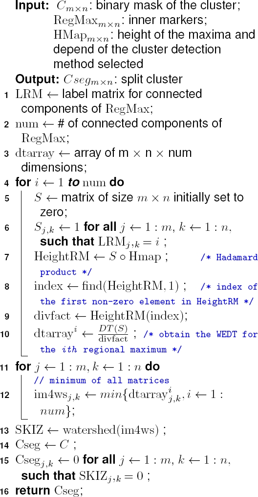
Then for each regional maximum its height value called divfact, is used to weight (divide) the EDT value associated to this maximum.
A three-dimensional array called dtarray is built in which its ith level is a matrix that contains the weighted EDT (WEDT ), which is the EDT with its values divided (weighted) by divfact.
The reasoning behind this procedure is that the WEDT value calculated in some specific point tends to be lower for a larger height of the maximum and viceversa.
This fact determines that the SKIZ lines tend to separate from higher maxima and come closer to lower maxima, and this leads to a better location of the SKIZ lines (equal distance) to segment clustered objects having different size.
The remaining i values give rise to matrices corresponding to each regional maximum, each one of them with its respective weight. The algorithm saves in dtarray the WEDT for each regional maximum in a cluster.
Then it computes the global WEDT map taking in each coordinate point of the image plane, the minimum value of the WEDT, calculated for all i saved in dtarray and saving it in im4ws matrix.
Then the marker controlled watershed transform is applied to this matrix to obtain the SKIZ lines which will be used to segment the binary cluster C.
Fig. 5 shows a block diagram illustrating the described algorithm, the pseudo code for it is shown above. Two alternative methods were compared with the proposed algorithm in other to explore their accuracy.
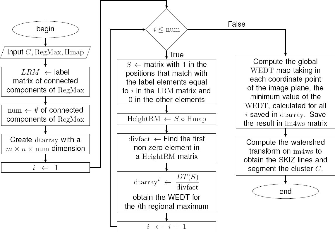
Fig. 5 Block diagram of the algorithm to segment the clusters using the Weighted External Distance Transform
These methods were the marker controlled watershed transform using the inner distance transform (CW ) and the marker controlled watershed transform using the external distance transform (EDT ).
The combination of the three methods implemented for the detection of clusters (Iterative H-maxima transform, Morphological filtering and Radon transform) with the three methods to split them into their constituent objects form nine combined methods.
Fig. 6 shows the result of the segmentation using the Iterative H-maxima method to detect markers and the three ways to split the cluster: the inner distance transform, the external distance transform and the proposed weighted external distance transform.
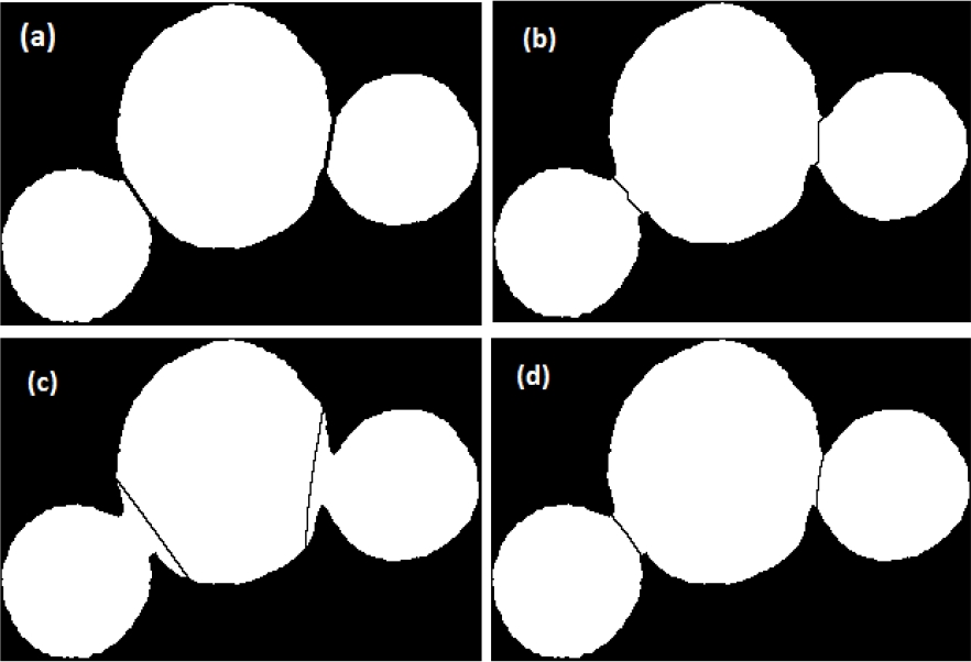
Fig. 6 Watershed lines in the segmentation result after detecting the clusters by means of iterative H-maxima algorithm. (a) Ground truth. (b) Using inner distance transform. (c) Using external distance transform. (d) Using the weighted external distance transform
In this figure, we can notice the difference in terms of the watershed lines. In (a) the ground truth lines (b) broken lines can be observed, in (c) the line is somewhat displaced from the right position and in (d) the splitting line appears in a right place.
2.6 Evaluating the Effectiveness of Clusters Detection
A comparison between the three methods to detect clusters allowed determining the most appropriate alternative.
This comparison considered the detection of clusters in terms of true positives (TP) or clusters classified as such, false positives (FP) single objects classified as clusters, true negatives (TN) single objects correctly classified, and false negatives (FN) as clusters classified as single objects. From these data, the indexes of effectiveness: sensitivity, specificity, accuracy, F-measure and precision were calculated.
These measures are defined as follows:
2.7 Evaluating the Segmentation Accuracy
The segmentation accuracy was tested using a ground truth composed by 500 binary clusters obtained from a first coarse segmentation, from which a careful, manually segmented version was built by digitally drawing an appropriate straight line between the vertices of the concavities that appear just at the points where the overlapping region of the roundish erythrocytes begin, as shown in Fig. 6a.
These clusters comprised two to eight single touching or overlapping objects with low to moderately different shapes, sizes and spatial orientations, up to 1220 single objects. The metric used to evaluate the accuracy of the segmentation was the Jaccard similarity index [10], which measures the coincidence between the segmentation result and the ground truth and is defined as:
where A and B are the binary sets to be compared and
The analysis and interpretation of the results when evaluating the Jaccard coefficients was performed applying statistical tests.
We compared the nine methods using the Friedman’s non-parametric rank test with a Bergmann and Hommel’s correction for the post-hoc analysis. These tests were computed using the public R scmamp package [5].
3 Results and Discussion
Fig. 7 shows two segmentation results using the HmaxWEDT method. Here the Iterative H-maxima transform is used to detect clusters and extract the inner markers and the weighted external distance transform (WEDT) to split the clusters into their constituent objects.

We stress the fact that this combination of methods obtained the best results. The effectiveness in the detection of clusters was measured in terms of sensitivity and specificity. We analyzed 43 images containing 4265 binary objects. Table 1 shows the indexes of effectiveness in the detection of clusters, for the three methods analyzed: Iterative H-maxima transform, Morphological filtering and Radon transform.
Table 1 Indexes of effectiveness in the detection of clusters
| Indexes | Iterative Hmax | Morph Filtering | Radon Transform |
| TP | 1057 | 1068 | 945 |
| TN | 3182 | 3181 | 3187 |
| FP | 2 | 3 | 0 |
| FN | 24 | 13 | 133 |
| Sensitivity | 97.78% | 98.8% | 87% |
| Specificity | 99.94% | 99.91% | 100% |
| F-measure | 98.79% | 99.26% | 93.43% |
| Accuracy | 99.39% | 99.62% | 96.88% |
| Precision | 99.81% | 98.72% | 100% |
The numbers in the tables were rounded to two decimal places. Table 2 shows the descriptive statistics of the Jaccard coefficients calculated for the nine methods analyzed, for which 1220 objects were used.
Table 2 Descriptive statistics of the Jaccard coefficient for the nine methods
| Method | Mean | Median | St.Dev. | Max | Min |
| HmaxCW | 0.946 | 0.948 | 0.01 | 0.965 | 0.853 |
| HmaxEDT | 0.985 | 0.991 | 0.021 | 1 | 0.749 |
| HmaxWEDT | 0.993 | 0.996 | 0.01 | 1 | 0.892 |
| MorphCW | 0.94 | 0.948 | 0.057 | 0.965 | 0.332 |
| MorphEDT | 0.977 | 0.991 | 0.055 | 1 | 0.157 |
| MorphWEDT | 0.987 | 0.994 | 0.042 | 1 | 0.393 |
| RadonCW | 0.946 | 0.948 | 0.017 | 0.965 | 0.561 |
| RadonEDT | 0.98 | 0.99 | 0.04 | 1 | 0.258 |
| RadonWEDT | 0.987 | 0.994 | 0.034 | 1 | 0.408 |
Here Hmax, Morph and Radon stand for the Iterative H-maxima transform, Morphological filtering and Radon transform respectively, and CW, EDT and WEDT for the classical watershed transform, external distance transform and weighted external distance transform.
This table shows that the method HmaxWEDT exhibited better results than the others, in terms of mean, median and standard deviation. Similar results were obtained with the other methods when using the WEDT.
The Friedman test found statistically significant differences in results among the compared algorithms with a p-value of 2.2e-16 (test statistic = 6234.5). Then, the Bergmann and Hommel post-hoc procedure was carried out in order to find which combination of methods showed a statistically significant difference.
As a further description in order to have a better understanding of the possible similarities and differences among the tested algorithms, we plotted and show in Fig. 8 a critical difference plot with the corrected p-value and
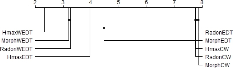
Fig. 8 Cross-comparison for the nine algorithms tested using the Friedman test and the Bergmann and Hommel post hoc correction. Groups of methods that are not significantly different appear connected by a horizontal line
In this plot, each algorithm is placed on an axis according to its average ranking. Then, those algorithms that do not show significant differences are grouped together using a horizontal line. The rankings in the plot assume that larger values have a poorer rank.
In our case, the plot shows that, in general, the HmaxWEDT combination method ranked significantly better than the other combined algorithms, showing as well statistically significant differences in comparison with the others.
Another representation of the results of this test is shown in Fig. 9, where in this graph each node represents an algorithm and shows its name and the computed Friedman’s test statistic.
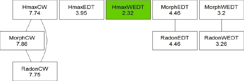
Fig. 9 Friedman test with the Bergmann and Hommel post hoc correction for the nine algorithms tested. Groups of methods that are not significantly different appear as connected nodes
A node with a filled background in green indicates the best ranked algorithm after this comparison. Lines between nodes indicate that the differences between connected algorithms are not found to be significant for α = 0.05, according to the Bergmann-Hommel post-hoc procedure.
There are no significant differences between the algorithms HmaxCW, MorphCW and RadonCW for which their mean ranks are very similar.
These three algorithms in spite of the way they use to detect the markers for the objects -using the methods Iterative H-maxima transform, morphological approach and Radon transform respectively- have in common the way used to split the clusters, e.g. using the classical watershed transform.
The same occurs with pairs MorphEDT and RadonEDT which use the external distance transform; and MorphWEDT and RadonWEDT which use the proposed weighted external distance transform.
3.1 Comparative Study
In order to make a comparative assessment of our proposed method, experimental results were compared to other state-of-art methods cited in the present article.
In spite that these works do not use the same database or even the same type of cells, the global results may provide an idea about how the figures obtained in the experiments reported in this article compare with those obtained in other works in this field.
In reference [18] the results are expressed in terms of percentages of correctly segmented clusters obtaining a 96.43% accuracy on cervical and breast cancer images.
The accuracy results obtained in our works are higher compared with this reference in spite that the image are from different types of cells. Reference [20] showed their results in terms of performance measures of overlapped cells detection as well as accuracy of splitting.
They achieved 97.4% accuracy in the overlapped cells detection on the test set. In our work, we obtain better results in the cluster detection process achieving 99.39% and 99.69% accuracy with the Iterative H-maxima transform and Morphological filtering methods respectively.
Reference [44] obtained high results in terms of sensitivity, precision and F-measure where true positive (TP) is the number of correctly split objects. Three datasets were used to evaluate the performance of the method and average values of sensitivity = 98.29%, precision = 99.02% and F-measure = 98.65% were obtained.
In our work, the TP is the number of objects classified correctly as clusters, and in this sense, we obtained 99.81% precision and 98.79% F-measure by the Iterative H-maxima transform method as well as 99.72% precision and 99.26% F-measure by the Morphological filtering method which are slightly better.
3.2 Runtime Analysis
This study was carried out using MATLAB (2016a version) on a computer with an Intel Core i3-2310M processor clocked at 2.10 GHz and with 4 GB of RAM and 64 bits Windows 10 Pro operating system. To reduce the computational load, the binary image obtained from the coarse segmentation was resized to resolutions of 1024 × 768 pixels.
Table 3 shows for one resized binary image the total of connected components (CC) and the indexes of TP, TN, FP and FN detected by the three methods. For this image, the Iterative H-maxima transform and Morphological filtering obtained the same results.
Table 3 Detection of cell clusters for one image Table 4. Mean runtime for each method (in seconds)
| Method | CC | TP | TN | FP | FN |
| Iterative H-maxima | 117 | 27 | 89 | 0 | 1 |
| Morph filtering | 117 | 27 | 89 | 0 | 1 |
| Radon transform | 117 | 23 | 89 | 23 | 5 |
These two methods exhibited the best results obtaining the TP and consequently the best results in terms of sensitivity, F-measure and accuracy showed earlier in Table 1.
Table 4 shows a comparison of the mean running times for the three clusters detection algorithms combined with the three methods used to split the clusters in their constituent parts.
Table 4 Mean runtime for each method (in seconds)
| Method | Radon | Morph Filtering | Iterative H-maxima |
| Classical Watershed transform (CW) | 8.66 | 1.82 | 46.41 |
| External distance transform (EDT) | 8.59 | 2.11 | 46.86 |
| Weighted external distance transform (WEDT) | 23.11 | 18.87 | 62.73 |
The morphological filtering method combined with the three cluster-splitting methods showed the best performance in terms of speed, which is a very important factor when analyzing large numbers of images.
The Iterative H-maxima method was the most time consuming. This result is a consequence of the need to perform a number of iterations calculating the H-maxima transform, which has a relatively high computational cost, in order to obtain the appropriate h values.
The same occurs with the WEDT method used to split the clusters. In this case, each detected cluster is to be analyzed to compute the weighted distance transform, which has a higher computational cost.
4 Conclusion
This research explored various alternatives to detect and split connected components in binary images, which appear in segmentation processes of microscopy images having touching or overlapping erythrocytes. The scope of this approach was constrained to blood smear images containing erythrocytes having moderate differences in size as well as a moderate degree of overlapping.
Three methods to detect connected components associated to clusters, named Iterative H-maxima transform, Morphological filtering and Radon transform were used, as well as three methods to split these connected components in their constituent parts, named in this case external distance transform (EDT ), the classical watershed transform (CW ) and the weighted distance transform (WEDT ) which result in nine possible combinations.

