


 text new page (beta)
 English (pdf)
 Article in xml format
 Article references
 Send this article by e-mail
 Cited by SciELO
  Similars in
SciELO
Similars in
SciELO 
 Permalink
1 Symbology
The following notation is used in the paper:
ω – |
Frequency, |
H(ω) – |
FRF system output, |
H – |
System operator, |
K – |
Inverse Volterra operator, |
W – |
Overall equalization system operator, |
ωn – |
Natural frequency, |
D – |
System input amplification, |
t – |
Time, |
y(t) – |
The output signal, |
yj(t) – |
Output signal from the j-th Volterra operator of the system, |
x(t) – |
Input signal, |
u(t) – |
System output acceleration, |
U(t) – |
The FRF of the output acceleration, |
z(t) – |
Output signal from the j-th inverse Volterra operator of the system, |
w(t) – |
Output signal from the j-th Volterra operator of the equalization system, |
i – |
square root of minus one, |
rj, pj, qj, uj1, j2, j3.... – |
ARX lags in time for y, x, errors, and powers of the output, |
kj, cj, gj, Aj – |
Modal parameters. |
2 Introduction
In previous work [1], an open-loop control was proposed for time-continuous nonlinear systems. This open-loop control is carried on by a Volterra inverse [2], whose operators are parametric models named Associated Linear Equations (ALE) [3]. They are the counterpart o de FRFs in the frequency domain as can be seen in [4, 5].
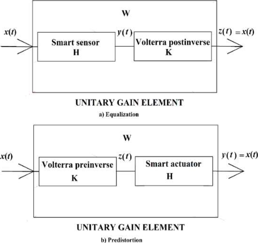
The principal characteristic of this method is that the whole system is transformed into an element of unitary gain and therefore losses are compensated, nonlinearities are eliminated and at least in theory, the array has infinite bandwidth.
The configuration for sensor systems (equalization strategy) can be seen in Figure 1. The Volterra inverse is connected in tandem with the sensor system.
To obtain a parametric model of a system is in the majority of practical cases very difficult if not impossible. Without a parametric model, it is not possible to obtain the ALEs.
A worthwhile option is the use of discrete models of the system such as the Nonlinear Autoregressive Moving Average with eXogenous inputs (NARMAX). A good introduction to this kind of model can be found in [6] and [7].
Some work on this kind of model and the Volterra series can be found in [6], where these models were applied to structural integrity. Recent applications have been done on ground vehicle control as in [8], though the present work offers a more explicit and simple means of control.
Other uses that can be mentioned are the simulation for system analysis with the aid of other methods of identification such as neural networks [9]. Several works focus on improving the model quality, including accounting for small changes in the system, e.g. [10, 11].
The main objective of this work is to present a novel construction of the inverse Volterra by discrete versions (AutoRegresive with eXogenous inputs ARX models) of the ALEs and to implement the control in a practical case.
The open-loop control is going to be implemented on an analogic Duffing oscillator. Some recent works on this kind of system can be found in [ & 13]. The Duffing oscillator is considered a sensor system and therefore an equalization strategy (Figure 1) is implemented.
A Duffing Oscillator is a very appropriate system for this kind of control as the number of Volterra operators is finite [14]. In practice, a traditional example of this kind of system are those structures that present softening or hardening stiffness, this kind of structures can be found for example in plane wings or helicopter propellers [15].
The work is organized into five sections. The first section is a breve description of the general theory of the ALEs and the inverse Volterra. The second section presents the novelty of this work, the discrete version of the ALEs for both direct and inverse systems. In the third section, the analogic Duffing oscillator is described. In the fourth section, open-loop control is implemented. The last section contains the conclusions.
3 Materials and Methods
3.1 Associated Linear Equations (ALEs)
In [3], it is explained that the most general second-order equation for which the Associated Linear Equations (ALEs) can be applied is:
Equation (1) includes two kinds of Volterra systems, the Duffing oscillator, and the Hammerstein. The Volterra series [2] decomposes the signal in an infinite series of operators:
Each operator corresponds to each harmonic output signal order. Where each operator is obtained from the Associated Linear Equations (ALEs). A Duffing oscillator is when in equation (1) one has P=1 and Q=0, e.g., a third-degree Duffing oscillator of is:
where N=3There is no intention to explain in detail how to obtain the ALEs from a parametric model, a detailed development is done in reference [2]. Here, it is only mentioned that those equations are obtained from a variation of the perturbation method, e.g., see [14]. In the same reference [2], it is demonstrated that all even-order Volterra operators of a third-order Duffing oscillator as that represented by equation (3) are null. The lower order non-null ALEs are:
Each equation in (4) represents a linear system that depends only on the nth-harmonic order of the input (as yi are a function of the nth-order frequencies of the input), which is obtained from products of lower-order operators.
3.2 Postinverse Volterra Operators by ALEs
The open-loop control that is used in this work [1] consists in connecting in tandem the system with its inverse Volterra (Figure 1). The basic theory can be seen in [15].
Let us represent the system operator as
Being x(t), w(t), and k(t) the respective outputs in the time domain,
where wj are the composed system [3]. In the most general case, there should be a maximum order N with significant contribution and therefore this is the maximum where wj is the composed system [3]. In the most general case, there should be a maximum order
From [15], the first-order inverse Volterra operators are defined as:
The second and third are respectively:
According to equation (8a), the second-order inverse operator is also null, as all the even direct operators of the Duffing oscillators of this kind (equation (3)) are null. The third-order Volterra inverse remains as:
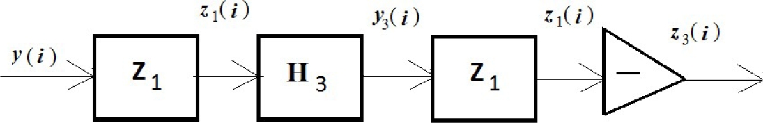
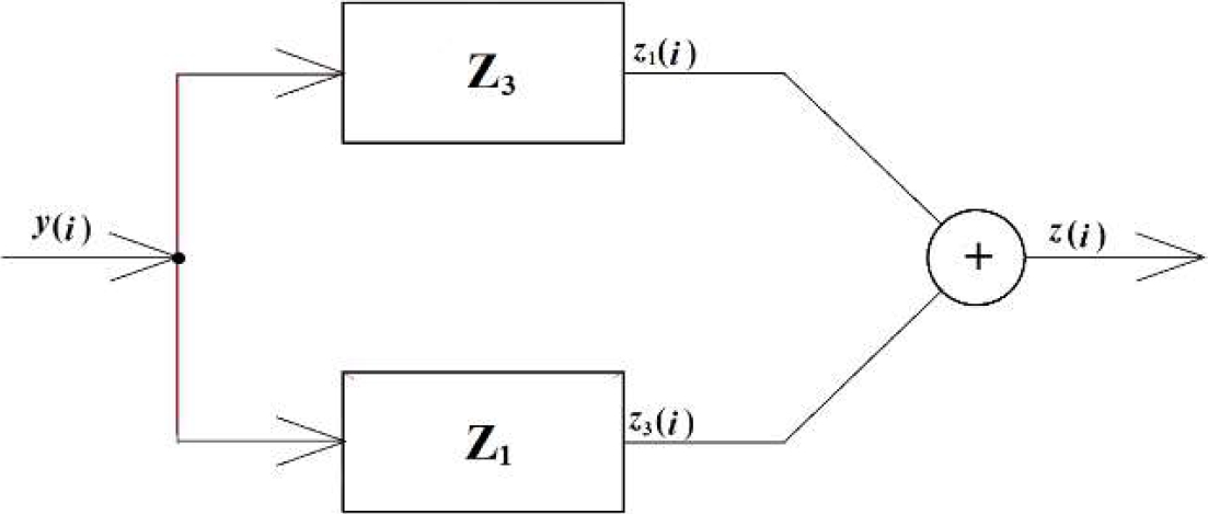
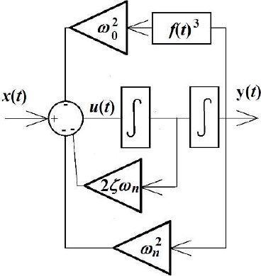
Figure 2 shows the block diagram. The output of the global operator
3.3 AutoRegresive with EXogenous Inputs (ARXs) Inverse Volterra Models
Now j, m, s are the lags with maximums of
A discrete Volterra series is:
substituting this equation into equation (11), we have:
where error terms are not included.
The Volterra series possesses a convergence maximum value xmax, so the input must comply with the following:
Under this value, it is the guarantee that:
Therefore, under these circumstances, it is always possible to cut the series up to an order k and then still have the required exactitude.
Taking as an example only the first three nonzero operators of equation (12).
The infinite sum is truncated up to three terms:
Developing the cube:
Equation (13) is then:
Using Fourier transform, it is possible to express any integrable function as a sum of complex exponentials. When rising this sum of exponential terms to any power generates terms function of harmonic frequencies (harmonic orders), that are the sum of the frequencies of the original terms.
As the equation (15) should remain valid at any time, the right and left sides have to remain the same for each harmonic order. Then the equation (15) can be split into several equations one contains all the harmonics of the same order. Equation (15) is split then in the following equations:
The equations above become the first, third, and fifth discrete (ARX) ALEs.
4 Results and Discussion
4.1 Discrete Volterra Inverse
This section is devoted to obtaining the inverse Volterra. The first inverse operator is easier to obtain in the frequency domain. The z-transform [16] of equation (16a) is:
where
H1(j) is then the ratio between the z-transforms of the output and input:
Considering equation (6), the inverse Volterra operator of the first-order is directly the inverse operator of the first-order Volterra operator of the systems
From equations (17) and (19):
Substituting equation (18) into (19):
This means that if the input is the first-order Volterra operator of the system (
Equation (21) can be also expressed as:
For completeness in the pre-inverse case (distortion strategy), the input into the equation (22) is
Now, equation (20) into equation (23) one obtains:
The z-inverse transform produces the first-order Volterra postinverse:
Something similar is obtained for the pre-inverse case, when the inverse transform on equation (23) gives:
About equation (25), in a real system, there are not such signals as y1(j) or y2(j), nor any other operator. Rather the system produces only the signal y(j) which is the sum of all these Volterra operators (equation 12). The real input into the first post-inverse operator is y(j). Then equation (25) has to be rewritten as:
Lets express equation (11) as:
After substitution in equation (27), one has (disregarding e terms):
Observe that in the particular case, in which the input signal is small enough so that only the first-order is significant, equation (25) is simply:
Therefore, z1(j)=x(j).
For the pre-inverse case, the input into the system, i.e., the input into the operator H is
Using equation (26) into (31):
Again, for a small enough signal, higher orders can be neglected, therefore:
As expected
The second-order operator from reference [15] shall be:
However, because
The third-order inverse operator
The input into the third-order operator for the post-inverse case is
Following equation (33), the signal goes through the direct operator H3, represented by equation (16b). Then, from equation (16a), the third-order input in H3 depends on powers of y1(i), then using equation (16a):
Again remember that the input into
That is the same equation as (11). Equation (16b) in the third-order inverse operator is simply:
Up to this point it has been solved up to
Using equation (35) one obtains:
Finally, from (30) z3(j) =- z1(j) therefore:
Adding equations (29) and (38) one obtains:
Then:
That according with equation (9) gives the expected result:
Observe that only two inverse operators suffice for obtaining as system exit x(j), no matter the input magnitude. It remains true meanwhile the physical elements of the system remain acting as a Duffing oscillator.
4.2 Inverse Series Convergence
Sometimes the inverse of Volterra presents instability. This section tries to find a suitable criterion to avoid this problem. Let's consider the following example of a simple linear ARX model:
Since it is linear, only the first-order Volterra operator is necessary. The inverse operator is:
Considering the initial condition for the inverse z1(1)=0 one has:
where y1(1) and y1(2) are system initial conditions.
For i=3 one has:
Substitution of equation (43) into equation (44):
The same procedure for the following two instants one has:
And
Generalizing for any instant i:
From equation (47) it can be observed that the inverse operator z1(i) is the function of powers of the ratio
In general, if there are more input lags, the criterion should be:
4.3 Duffing Oscillator Model
In [8], Duffing oscillator model was identified and the following equation is obtained:
As can be seen, the coefficients of the input lags (
The Duffing oscillator does not possess a second power term (equation (40)). It implies that it has only even-order non-zero operators. As it was done in section 2.3, the first three non-zero operators are obtained:
Equations (50) are obtained in the same way as equations (16). The input signal into the Duffing oscillator system is a random signal with an rms of 13.55 units. The system is simulated, and in Figure 4, the comparison between the input and the output signal is shown.
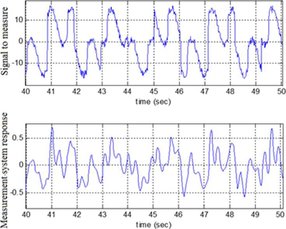
Because of the system inertia, nonlinearity, and noise, the difference between both signals is quite noticeable, i.e., the measurement signal differs greatly from the actual signal to be measured.
Now, let us implement the equalization strategy for controlling the measuring system (the Duffing oscillator equation (50)).
By the use of equation (16) and by the same process done in section 3.1, the first inverse of the Volterra operator is:
By the use of equations (50) and (51) on equation (33) the signal
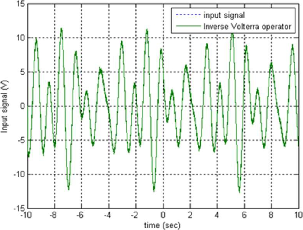
Figure 5 is again compared to the input signal, but this time with the output produced by the equalization control. It is now very difficult to see visually the difference between the input signals

Fig. 5 Output of the equalization system (Duffing oscillator-Post-inverse Volterra) compared with the system input (signal to measure)
The Frequency Response Function (FRF) of the first order of the Duffing oscillator is shown in Figure 6.
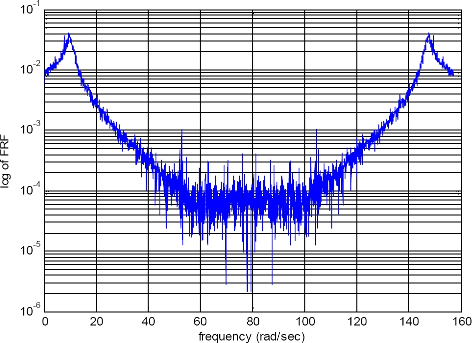
The semilogarithmic graph shows a bandwidth of 30rad/sec. It implies that if the input signal is of a frequency of 200rad/sec the Duffing oscillator is not going to be capable to measure such a signal. This circumstance can be verified in Figure 7, where a signal of a frequency of 200 rad/sec is measured. The Duffing oscillator response is indistinguishable in the graphic.
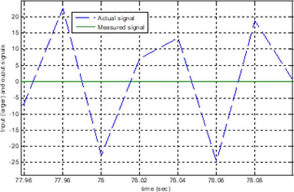
Fig. 7 For very high frequencies, the Duffing oscillator used as a measurement system has very low response
Now, if the signal is measured with the equalization strategy, the result is shown in Figure 8. What is now indistinguishable is the difference between the signal to be measured x(i) and the measured signal w(i). The mse is only 0.192%.

4.4 Analog Duffing Oscillator System
An analog electronic system is used in this work. It is designed as a third-degree Duffing oscillator, see equation (3). This equation can be rewritten in an integral form as in [9]:
The design of integral blocks is reported to have more stability than a design with derivative elements. Figure 9 shows a schematic of the system. The Fourier transform of equation (30) for the first-order is:
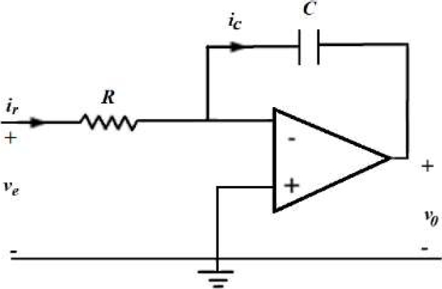
The integration blocks are constructed traditionally by Op-amps (Figure 10). The cubic operator is done by connecting in cascade three multiplicative circuits AD633JN/AN. The electronic design can be seen in Figure 11.

4.4.1 Identification
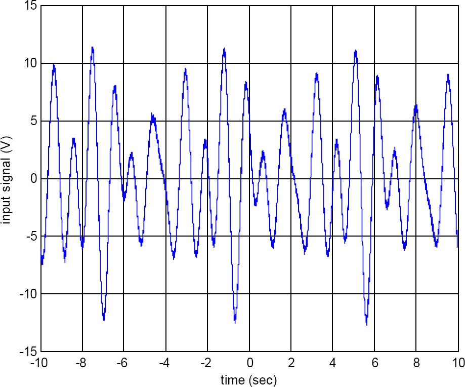
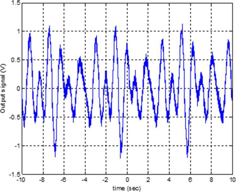
The input into the system is a three-harmonic signal shown in Figure 12. The system response is shown in Figure 13 The input frequencies are 6, 12, and 15 rad/sec. The output is filtered; this is to eliminate frequencies bigger than 50rad/sec, to prevent noise contamination. The data is taken at an interval of 0.02 sec.
The NARX model proposed for this system is:
Applying a NARX system identification procedure [12], the model found is:
Figure 14 compares the simulation output from the NARX model (equation (54)) and the real system response, the mse is 5.143%. The analog system presents certain instabilities both in frequency and in amplitude that implies that any model in equation (45) can be used only up to an input amplitude of 13 V and a frequency of 60rs/sec.
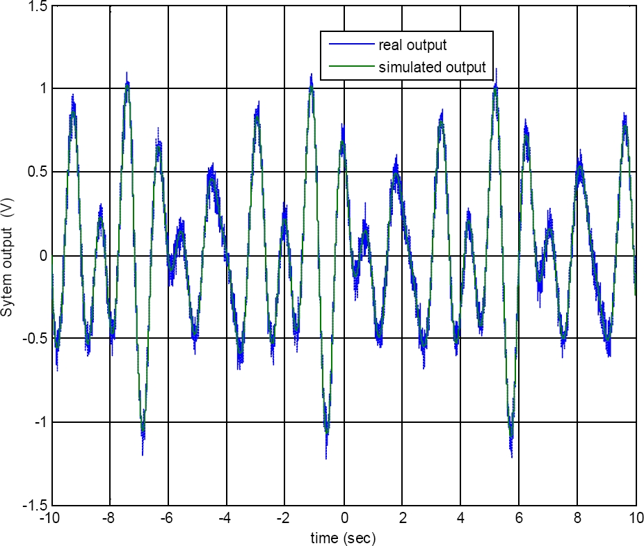
Fig. 14 Comparison between the output of the Duffing oscillator system signal and that obtained by the NARMAX model
This limitation is not associated with predistortion control, but with the change in the response behavior of the elements of the analog system.
Just as equations (16) were obtained, the first three non-zero ALE's are: Only the first three ALEs are obtained as the inverse Volterra is composed only for the first three order inverse operators.
It is possible to compare the ARX obtained, i.e., the ALE´s with the real corresponding response of the system. The whole signal is supposed to contain all the nth-order signals.
If equation (55a) is subtracted from the output signal, the results are very close to the sum of the harmonic signals of the second harmonic order onwards.
The adequate amplitude of the input signal gives a signal dominated by the second harmonic order signal.
Now, subtracting the equation (55b) from this signal, the signal that results is mainly the third harmonic order.
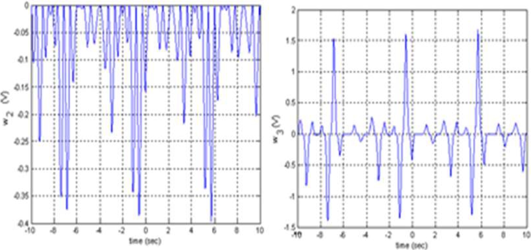
It is possible then to compare each harmonic signal of the output system with the corresponding ALE (equations (55)) see Figure 14.
Figure 15b shows that the curves differ from each other. This is because the third-order signal is of significant magnitude when compared with the second-order.
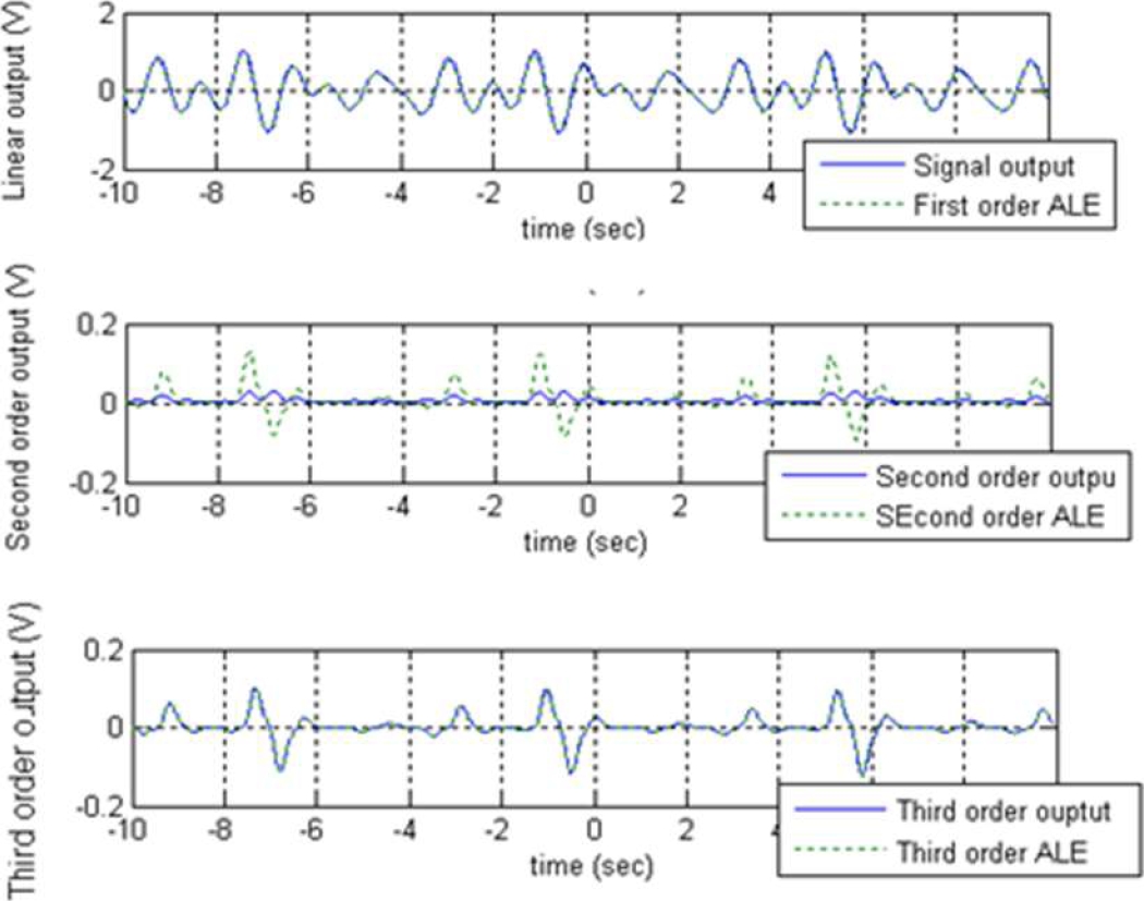
However, the remaining signal is quite close to the third-order ALE and therefore the ALEs are correct:
4.5 inverse Volterra Model for the Analog Duffing Oscillator System
From equation (20) and the system model (54), the first inverse Volterra frequency response function model is obtained by the z-transform as:
The corresponding ARX model is.
The second-order operator is according to [2] (see equation (31)):
The third-order inverse Volterra operator is now:
That differs from equation (33) because the second-order operator is not zero in this case. Figure 16 shows the plot of the second and third-order Volterra inverse operators. The equalization strategy is implemented and then the signal that results is shown in Figure 17. The mean square error (mse) between these two signals is only 3.0%. The output signal is quite the same as the signal to measure.
5 Conclusions
Two main objectives have been pursued in this work. The first one is to apply for the first time the equalization strategy on a practical system and on the other hand to present the discrete version of the Associated Linear Equations (ALEs) for both direct and inverse Volterra operators. Two systems were considered: a Duffing oscillator NARMAX model with additive noise and an analog system.
Duffing oscillator system is considered to follow the dynamics of a sensor system.
The equalization strategy of control is implemented for both systems using the discrete version of the inverse Volterra operators. In both cases, the original signal (the signal to be measured) is accurately obtained.
For the simulated system, it was possible to verify an infinite band wide. In the analog system is not possible to do the same, because the elements of the system are not stable at all frequencies and then the Duffing oscillator response is lost.
The use of the Volterra inverse seems to be very promising for systems where feedback is not an alternative, such as measuring and actuator systems.
In both cases, the nonlinearities and the inertia of both systems are eliminated and both systems act as elements of unitary gain just as expected.

