Articles of the thematic section
Computing the Clique-Width on Series-Parallel Graphs
Marco Antonio López-Medina1
*
J. Leonardo González-Ruiz1
J.Raymundo Marcial-Romero1
J. A. Hernández1
11 Universidad Autónoma del Estado de México, Facultad de Ingeniería, Mexico. jlgonzalezru@uaemex.mx, jrmarcialr@uaemex.mx, xoseahernandez@uaemex.mx.
Abstract:
The clique-width (cwd) is an invariant of graphs which, similar to other invariants like the tree-width (twd) establishes a parameter for the complexity of a problem. For example, several problems with bounded clique-width can be solved in polynomial time. There is a well known relation between tree-width and clique-width denoted as cwd(G)≤3⋅2twd(G)−1. Serial-parallel graphs have tree-width of at most 2, so its clique–width is at most 6 according to the previous relation. In this paper, we improve the bound for this particular case, showing that the clique-width of series-parallel graphs is smaller or equal to 5.
Keywords: Graph theory; clique-width; tree-width; complexity; series-parallel
1 Introduction
The clique-width is an invariant which set up a parameter to measure the complexity of a problem. Computing the clique-width consists on finding an algebraic finite term which represents in a succinct way the graph, meaning that its operations establishes how to built the graph. Courcelle et al. [3] present a set of four operations to built the algebraic expression called a term: 1) label creations which represent a vertex, 2)disjoint unions among graphs, 3) edge creation and 4) vertex re-label. The number of labels used to built a finite term is commonly denoted by k. The minimum number k used to built the term, also called k-expression, defines the clique-width.
Finding the smallest k which minimize the k-expression is an NP-Complete problem [7].
It has been observed that if the clique-width increases for a certain class of graphs then the complexity of a given problem for such a class of graphs also increases since the difficulty to decompose the graph increases. In recent years, clique-width has been studied in different class of graphs showing the behaviour of this invariant under certain operations.
Recent research shows how to calculate the clique-width in special types of graphs, for example in [12] prove that (4k1,C4,C5,C7)-free graphs that are not chordal have unbounded clique-width. Also in [5] a complete classification of graphs H was obtained, they shown that for these graph classes, a well-quasi-orderability implies boundedness of clique-width.
In [10], it is shown that the clique-width of Cactus graphs is smaller or equal to 4 and is presented a polynomial time algorithm which computes exactly a 4-expression. Also in [9] it is shown how to compute the cwd of Polygonal Tree Graphs and is presented a polynomial time algorithm which computes the 5-expression.
In a similar way, another invariant of graphs is tree-width [8], however, cwd is more general than tree width in the sense that, graphs with small tree-width also have small cwd.
A special class of graphs are the so called series-parallel graphs which can be obtained by recursive applications of series and parallel connections [6, 11]. This kind of graphs are a subclass of what are called planar graphs.
In this paper we show how to built a series-parallel graph and later on the algebraic 5-expression which defines the cwd, so we show that the cwd of a series-parallel graph is 5 improving the best known bound known of 6 [2].
The structure of the paper is as follows: section 2 presents the preliminaries of the paper, in section 3 the main result is demonstrated, an algorithm to compute the clique-width is shown in section 4. Finally, the conclusions are established in section 5.
2 Preliminaries
2.1 Graph
A graph G is denoted by G=(V(G),E(G)), where V(G) is the set of vertices in G and E(G) the set of edges in G. A path graph is denoted as a set of connected vertices that have two end points and every inner vertex xi have exactly two incident edges, d(xi)=2.
2.2 Series-Parallel Graph
A graph is series-parallel if it can be built from a single edge and the following two operations:
series construction: subdividing an edge in the graph.
parallel construction: duplicating an edge in the graph.
Another characterization of a series-parallel graph is that it do not contain a subdivision of k4 (complete graph of 4 vertices).
As the first characterization of series-parallel graphs implies, a series-parallel graph always has a vertex of degree two, although series-parallel operations may construct multiple edges, in this paper we only work with simple graphs.
2.3 Clique-Width
We now introduce the notion of clique-width (cwd, for short). Let  be a countable set of labels. A labeled graph is a pair (G,γ) where γ maps each element of V(G) into
  . A labeled graph can also be defined as a triple G=(V(G),E(G),γ(G)) and its labeling function is denoted by γ(G). We say that G is C-labeled if C is finite and γ(G)(V)⊆C. We denote by
  (C) the set of undirected C-labeled graphs. A vertex with label a will be called an a-port. We introduce the following symbols:
— a nullary symbol a(v) for every a∈ and v∈V;
— a unary symbol ρa→b for all a,b∈  , with a≠b;
— a unary symbol ηa,b for all a,b∈  , with a≠b;
— a binary symbol ⊕.
These symbols are used to denote operations on graphs as follows: a(v) creates a vertex with label a corresponding to the vertex v, ρa→b renames the vertex a by b,ηa,b creates an edge between a and b, and ⊕ is a disjoint union of graphs.
For C⊆  we denote by T(C) the set of finite well-formed terms written with the symbols ⊕, a, ρa→b, ηa,b for all a,b∈C, where a≠b. Each term in T(C) denotes a set of labeled undirected graphs. Since any two graphs denoted by the same term t are isomorphic, one can also consider that t defines a unique abstract graph.
The following definitions are given by induction on the structure of t. We let val(t) be the set of graphs denoted by t.
If t∈T(C) we have the following cases:
t=a∈C: val(t) is the set of graphs with a single vertex labeled by a;
t=t1⊕t2: val(t) is the set of graphs G=G1∪G2 where G1 and G2 are disjoint and G1∈val(t1), G2∈val(t2);
t=ρa→b(t′): val(t)={ρa→b(G)|G∈val(t′)} where for every graph G in val(t′), the graph ρa→b(G) is obtained by replacing in G every vertex label a by b;
t=ηa,b(t′): val(t)={ηa,b(G)|G∈val(t′)} where for every undirected labeled graph G=(V,E,γ) in val(t′), we let ηa,b(G)=(V,E′,γ) such that:
E′=E∪{{x,y}|x,y∈V,x≠y,γ(x)=a,γ(y)=b}, e.g. ηa,b(G) adds an edge between each pair of vertices a and b in G.
For every labeled graph G we let:
cwd(G)=min{|C||G∈val(t),t∈T(C)}.
A term t∈T(C) such that |C|=cwd(G) and G=val(t) is called optimal expression of G [4] and written as |C|-expression.
In other words, the clique-width of a graph G is the minimum number of different labels needed to construct a vertex-labeled graph isomorphic to G using the four mentioned operations [1].
3 Computing cwd(G) when G is a Series-Parallel Graph
In this section we show the k-expression for series and parallel graphs independently and later on how to combine them in order to present the 5-expression for series-parallel graphs. We firstly begins with series graphs. Although the result for this kind of graphs is well-known, we need a special construction to combine them with parallel graphs.
Lemma 1 If G is a series graphs (a path graph) then cwd(G)≤4.
Proof 1 Let G be a series graph, which is denoted as follows:
1 ————— 2 ————— 3 ————— 45 – – – – n
The k-expression is built as follows:
|
k − expression
|
Graph G
|
Labels |
| kG=η(a,b)(a(1)⊕b(2)) |
a(1) ------------ b(2) |
2 |
| kG=η(b,c)(kG⊕c(3)) |
a(1) - b(2) - c(3) |
3 |
| kG=η(c,d)(kG⊕d(4)) |
a(1) - b(2) - c(3) - d(4) |
4 |
| kG=ρc→b(kG) |
a(1) - b(2) - b(3) - d(4) |
3 |
| kG=ρd→c(kG) |
a(1) - b(2) - b(3) - c(4) |
3 |
| kG=η(c,d)(kG⊕d(5)) |
a(1) - b(2) - b(3) - c(4) - d(5) |
4 |
| kG=ρc→b(kG) |
a(1) - b(2) - b(3) - b(4) - d(5) |
3 |
| kG=ρd→c(kG) |
a(1) - b(2) - b(3) - b(4) - c(5) |
3 |
| ⋮ |
|
|
| kG=η(c,d)(kG⊕d(n)) |
a(1) - b(2) - b(3) - b(4) - c(5)−d(n) |
4 |
| kG=ρc→b(kG) |
a(1) - b(2) - b(3) - b(4) - b(5)−d(n) |
3 |
| kG=ρd→c(kG) |
a(1) - b(2) - b(3) - b(4) - b(5)−c(n) |
3 |
4 labels are used to built a series graph. At the end of the process we relabel the end vertices as a and c respectively, while the rest of the vertices are assigned label b, this assignment will be used at the end of each proof in the rest of the paper.
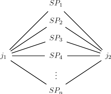
Lemma 2 If G is a parallel graph formed by series subgraphs then cwd(G)≤5.
Proof 2 Let n be the number of series subgraphs which forms the parallel graph:
By lemma 1, each k-expression of s1,s2,s3…sn requires 3 labels, let says a, b and c. Let a and c be the end vertices of each one. If j1 and j2 are the union vertices the final k-expression is given by:
kG=η(c,e)(η(a,d)(ks1⊕ks2⊕ks3⊕ks4⊕⋯ksn⊕d(j1)⊕e(j2)))
kG=ρe→c((ρc→b((ρd→a((ρa→b(kG))))
Although 5 labels are needed, in the last steps the joint vertices j1 and j2 are labeled with a and c respectively and the rest of the vertices are labeled with b.
A series-parallel graph can be composed by the following rules:
— A simple path is series-parallel (SP), Lemma 1.
— A parallel graph formed by series subgraphs is series parallel (SP). Lemma 2.
-
— if SP1 and SP2 are series parallel graphs then:
– The path graph formed by SP1,SP2,…,SPn is series parallel (SP). Lemma 5.
– The parallel graph formed by SP1,SP2,…,SPn with union points j1,j2 is series parallel (SP). Lemma 3.
– The parallel graph formed by SP2,SP3,…,SPn with union points SP1,j1 is series parallel (SP). Lemma 4.
Lemma 3 Let G a series-parallel graph which is connected to an other series-parallel graph, then the cwd(G)≤5.
Proof 3 Let G a parallel graph as follows:
SP1 —————————— SP2
Where SP1 and SP2 are series-parallel graphs and j1 is a joint vertex. By lemma 2 shows how to build the k-expression of SP1 and SP2 respectively.
kG=η(d,e)((ρc→d(kSP1))⊕(ρa→e(kSP2)))
kG=ρd→b(ρe→b(kG))
The initial vertex of SP1 and the final vertex of SP2 are labelled by a and c respectively, while the rest of the vertices correspond to the label b.
Lemma 4 If G is a graph which contains series-parallel subgraphs then cwd(G)≤5.
Proof 4 Let n be the number of series-parallel subgraphs which forms the parallel graph where n≥0:
By lemmas 1, 2, 3, each k-expression of SP1,…,SPn requires 3 labels, let says a, b and c. The end vertices of each one are a and c. If j1 and j2 are the union vertices the final k-expression is given by:
kG=η(c,e)(η(a,d)(kSP1⊕⋯⊕kSPn⊕d(j1)⊕e(j2)))
kG=ρe→c((ρc→b((ρd→a((ρa→b(kG))))
The end vertices j1 and j2 are labeled with a and c respectively and the rest of the vertices are labeled with b.
Lemma 5 Let G be a parallel graph with end points SP1 and j1 and elements SP2,SP3,…,SPn.
Proof 5 By lemmas 1, 2, 3 and 4, we know the k-expression of SP1 and each k-expression of SP1,…SPn requires 3 labels, let says a, b and c. The end vertices of each one are a and c:
kG=η(e,d)(ρa→d(kSP2⊕⋯⊕kSPn))⊕(ρc→e(kSP1)),
kG=ρd→c(ρc→b(η(c,d)((ρd→b(ρe→b(kG)))⊕d(j1)))).
The initial vertex of SP and the joint vertex j1 are labelled by a y c respectively, while the rest of the vertices correspond to the label b.
Lemma 5 can be applied transitively, e.g. j1 to the left and SP1 to the right.
Theorem 1 Let G a series-parallel graph, the cwd(G)≤5.
Proof 6 By series-parallel definition lemmas 1, 2 , 3, 4 and 5 allow to built any series parallel graph so cwd(G) is ≤5
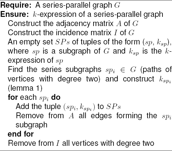
4 Algorithm to Compute cwd of Series-Parallel Graphs
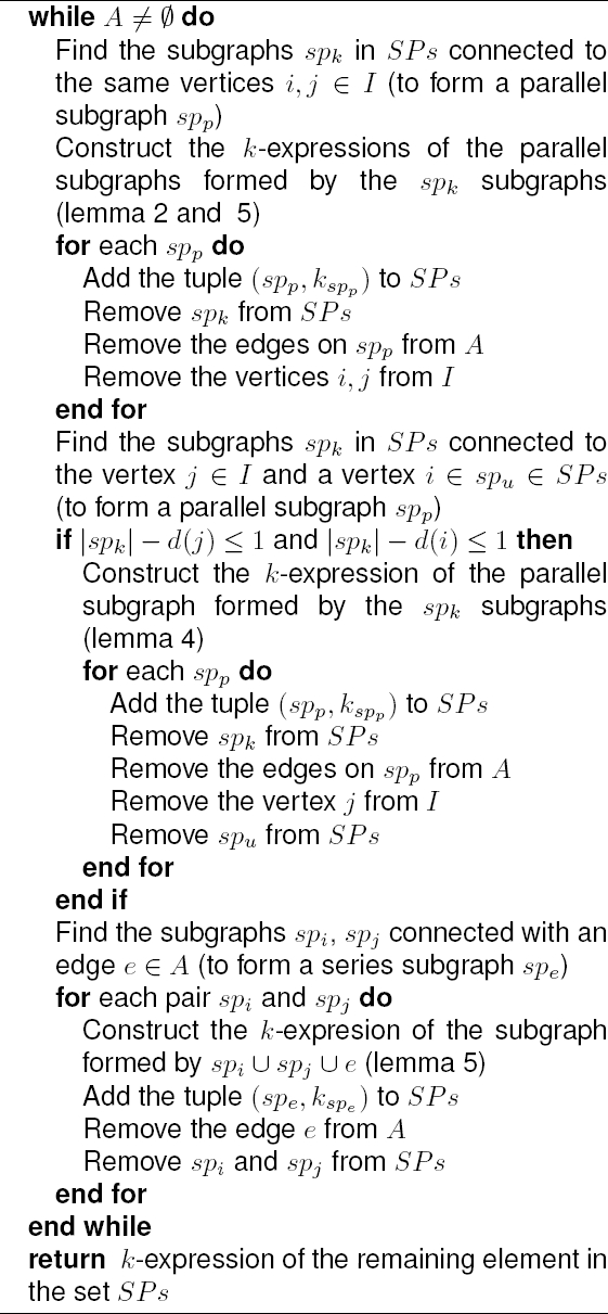
The construction of the k-expression of a series-parallel graph is presented in Algorithm 1 and 2.
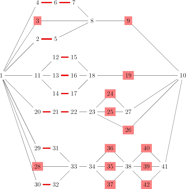
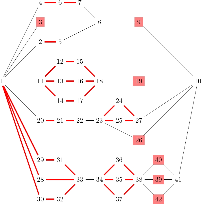
We explain the algorithm with the following example:
Given a series-parallel graph:
With the adjacency matrix A, the incidence matrix I and the set SPs.
First lines from 3 to 9 allow to construct the spi subgraphs, formed by paths of vertices with degree two, using lemma 1.
From line 11 to 18 we construct the parallel graphs with the joint vertices we have in I (lemma 2 and 5).
From lines 19 to 29 we can construct a parallel graph with joint vertex and a vertex on a spk subgraph (lemma 4). Notice that the end point 1 and 8 cannot be added at this time since the degree of 1 will not be 0 after joining it to the subgraphs.
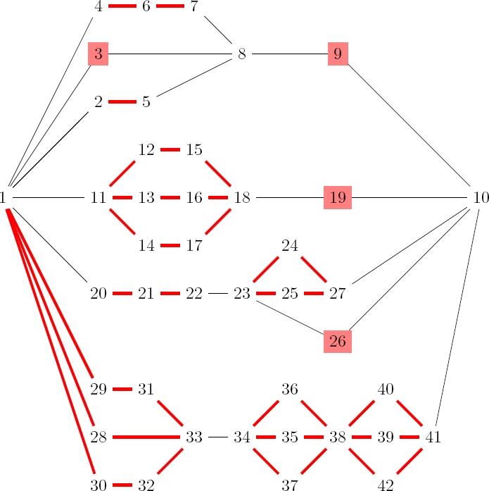
From lines 30 to 36 we can connect two spi and spk subgraphs by an edge in A (lemma 5).
From lines 19 to 29 we can construct a parallel graph with joint vertex and a vertex on a spk subgraph (lemma 4).
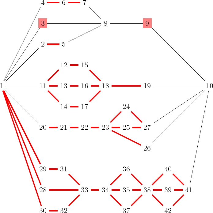
Again, from lines 19 to 29 we can construct a parallel graph with joint vertex and a vertex on a spk subgraph (lemma 4).
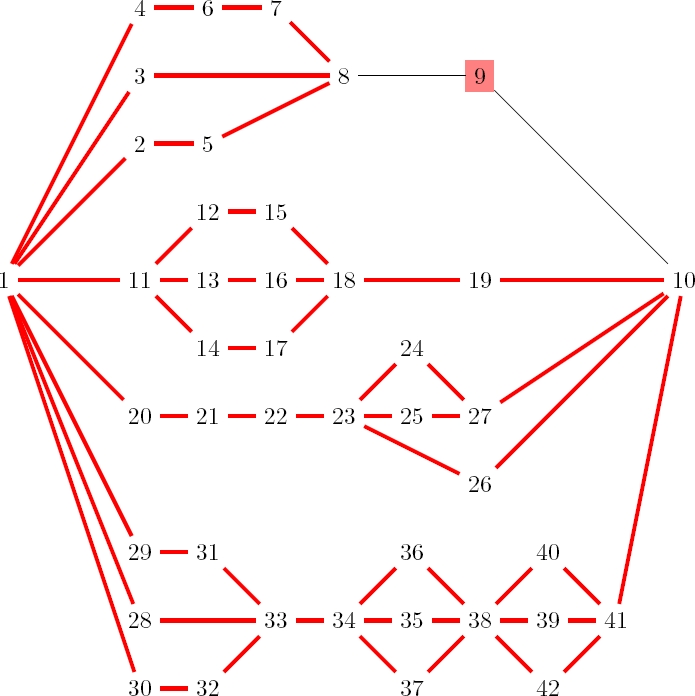
Finally, from lines 30 to 36 we can connect two spi and spk subgraphs by an edge in A (lemma 5).
As a result of the algorithm we have a unique element sp∈SPs with the k-expression that represents it.
5 Conclusions
In this paper we show that five labels are enough to compute the clique-width of series-parallel graphs instead of six labels as Courcelle et al. [2] shown. Our main proof is based on the series-parallel graph’s definition which consists on building this kind of graph from series subgraphs joined by vertices which form parallel components. An algorithm was presented with time complexity O(n2).
References
1. Bonomo, F., Grippo, L. N., Milanic, M., Safe, M. D. (2016). Graph classes with and without powers of bounded clique-width. Discrete Applied Mathematics, Vol. 199, pp. 3–15. Sixth Workshop on Graph Classes, Optimization, and Width Parameters, Santorini, Greece, October 2013.
[ Links ]
2. Corneil, D. G., Rotics, U. (2001). Graph-Theoretic Concepts in Computer Science: 27th InternationalWorkshop, WG 2001 Boltenhagen, Germany, June 14–16, 2001 Proceedings, chapter On the Relationship between Clique-Width and Treewidth. Springer Berlin Heidelberg, Berlin, Heidelberg, pp. 78–90.
[ Links ]
3. Courcelle, B., Engelfriet, J., Rozenberg, G. (1993). Handle-rewriting hypergraph grammars. Journal of Computer and System Sciences, Vol. 46, No. 2, pp. 218–270.
[ Links ]
4. Courcelle, B., Olariu, S. (2000). Upper bounds to the clique width of graphs. Discrete Applied Mathematics, Vol. 101, pp. 77–114.
[ Links ]
5. Dabrowski, K. K., Lozin, V. V., Paulusma, D. (2020). Clique-width and well-quasi-ordering of triangle-free graph classes. Journal of Computer and System Sciences, Vol. 108, pp. 64–91.
[ Links ]
6. Dieter, J. (2013). Graphs, Networks and Algorithms. Springer Publishing Company, Incorporated, 4th edition.
[ Links ]
7. Fellows, M. R., Rosamond, F. A., Rotics, U., Szeider, S. (2009). Clique-width is np-complete. SIAM Journal on Discrete Mathematics, Vol. 23, No. 2, pp. 909–939.
[ Links ]
8. Fomin, F. V., Golovach, P. A., Lokshtanov, D., Saurabh, S. (2010). Intractability of clique-width parameterizations. SIAM Journal on Computing, Vol. 39, No. 5, pp. 1941–1956.
[ Links ]
9. González-Ruiz, J. L., Marcial-Romero, J. R., Hernández, J. A., De Ita, G. (2017). Computing the clique-width of polygonal tree graphs. Pichardo-Lagunas, O., Miranda-Jiménez, S., editors, Advances in Soft Computing, Springer International Publishing, Cham, pp. 449–459.
[ Links ]
10. González-Ruiz, J. L., Marcial-Romero, J. R., Hernández-Servín, J. (2016). Computing the clique-width of cactus graphs. Electronic Notes in Theoretical Computer Science, Vol. 328, pp. 47–57. Tenth Latin American Workshop on Logic/Languages, Algorithms and New Methods of Reasoning (LANMR).
[ Links ]
11. Gross, J. L., Yellen, J., Zhang, P. (2013). Handbook of Graph Theory, Second Edition. Chapman & Hall/CRC, 2nd edition.
[ Links ]
12. Penev, I. (2020). On the clique-width of (4k1,c4,c5,c7)-free graphs. Discrete Applied Mathematics, Vol. 285, pp. 688–690.
[ Links ]


 text new page (beta)
 English (pdf)
 Article in xml format
 Article references
 Send this article by e-mail
 Cited by SciELO
  Similars in
SciELO
Similars in
SciELO 
 Permalink