1 Introduction
Problems of reaching agreement are central to distributed computing. Often consensus is needed to agree on the same value, for example, when agents need to agree on whether to commit or abort the results of a distributed database transaction. However, in many situations consensus is impossible to achieve, such as networks where agents may crash and delays are unpredictable [15], or read/write shared memory models [22], or certain dynamic networks [11]. All these impossibility results are due to the same reason: the indistinguishability graph [2] of the global states of a protocol trying to solve consensus is connected, while that of the consensus task is not [5, 18, 23].
In this paper we are interested in many other situations, where approximate agreement is sufficient; for example, when sensors estimate a certain measurement or clock synchronization where agents maintain similar time estimates. Many variants of approximate agreement, and in various message passing and shared memory models have been considered since early on, e.g., [14].
Approximate agreement is an interesting weakening of consensus that can be solved in many more situations. The task is parametrized by a real number ε>0, and the agents must decide values that are at most ε away from each other. The time to reach a decision however, will be a function of how small ε is. Many algorithms have been proposed to try to minimize the time until decision is reached, e.g. in shared memory models [20], in networks [10], and others.
Consensus has been thoroughly studied from the epistemic logic perspective, and the close connection with common knowledge is well-known [24]. Approximate agreement has been less studied from the epistemic logic perspective. It was recently shown that it is closely related to k-iterated knowledge in a certain shared memory model [25], roughly, meaning that the agents must know, that they know, that they know that they know, and so forth (k times), each other’s inputs, in order to reach certain degree of approximation of their decisions. This was shown within a general simplicial complex model for multi-agent epistemic logic for task solvability. In this paper we are interested in studying in more detail this result, as well as providing a self-contained, more elementary introduction to the topic.
We focus on one specific distributed computing model, that has received much attention recently, dynamic networks (see surveys [6, 8, 21, 27]). There is a fixed set of agents that operate in rounds communicating by sending messages to each other. Rounds are synchronous in the sense that the messages received at some round have been sent at that round. At each round, the communication graph is chosen arbitrarily among a set of directed graphs, G. This set G determines the network model. Hence the communication graph can change unpredictably from one round to the next.
Dynamic networks are interesting for various reasons, in particular because they include as special cases other classic models, such as shared memory models [19], so results in dynamic networks can often be extrapolated to other models.
Approximate agreement is solvable in a dynamic network model G if and only if each communication graph in G has a rooted spanning tree [9] (e.g. [5, 7]). In this work we consider such a G, where approximate agreement is solvable, but not consensus. Two agents, starting with binary input values, are to decide values in the interval of their inputs, which are at most 1/3k apart from each otherfn. We rephrase this problem epistemically, as requiring that the agents reach k-iterated knowledge about their respective inputs. This knowledge can be achieved, if and only if, the protocol runs for k rounds. We show these results in the dynamic epistemic logic (DEL) [4] framework of [25], instantiated to a dynamic network. We follow recent work, in using the dual of a Kripke graph, a simplicial complex, as a model for multi-agent epistemic logic, that exposes the topological features that determine if a task is solvable [17, 26]. While the results we present here have been shown in these papers, we instantiate the results using graphs instead of simplicial complexes, making the development more accesible.
Organization. Before getting into epistemic logic, in Section 2 we present two algorithms that solve approximate agreement. In Section 3 we overview the DEL framework. In Section 4 we give the formal epistemic logic semantics to our dynamic network model, and we do the same for tasks, in Section 5. The solvability results are in Section 6. The conclusions are in Section 12. Additional details and proofs are in the Appendix.
2 Approximate Agreement Algorithms
We start by presenting algorithms, to guide the reader’s intuition before diving into the formal semantics considerations of the subsequent sections.
Two agents, g, w (for gray, white), communicate with each other exchanging messages in a sequence of k rounds. In a round, each agent sends a message to the other agent, receives the message sent by the other agent, and then updates its local state. In each round, at most one of the two messages sent may be lost.
Let N=3k, k≥0. In the N-approximate agreement task, after k rounds, agents decide values dg, dw, resp., of the form i/N, for an integer i, 0≤i≤N. Each agent starts with an input value from the set {0,1}:
The decisions must be such that if the two input values are equal, then both output values are equal to the input value. Otherwise, the output values dg, dw satisfy |dg−dw|≤1/N. The algorithm in Figure 1 solves N-approximate agreement in k rounds (e.g [10, 16] and [18] Chapter 2). A simple induction argument on the number of rounds proves its correctness. The examples on the right show two 4-round executions where agents agree on values 1/34=1/81 from each other. The first example (represented in the top two rows) represent an execution where all messages from w are lost. The first column, with labels 0 and 1, corresponds to the initial input values. Then each subsequent column shows the values of the processes after each round. An edge indicates that a message was received. In the second execution (bottom two rows of the picture), both messages arrive in the first two rounds, but in the 3rd round the message from g to w is lost, and in the 4th round the message from w to g.
The algorithm of Figure 1 can be used by the agents to decide values arbitrarily close to each other, by running enough rounds, k. However, the size of messages sent grows with k. Remarkably, there is an algorithm that solves the problem sending 1-bit messages, see Figure 2, which is a reformulation and small adaptation of the algorithm given in [12]. In a 1-bit protocol, each message received from the other process can be either 0, 1 or ⊥. Thus, in a k-round computation, we call the view of a process the sequence v∈{0,1,⊥}k of messages that were received. For instance with four rounds, v=(0,0,⊥,1) indicates that the process received message “0” in the first two rounds, no message in the third round, and message “1” in the fourth round. To reduce notation, we often write such a view as a word, e.g. v=00⊥1. Given a view v and a message m∈{0,1,⊥}, we write v⋅m for the new view where we append m at the end of v.
The algorithm in Figure 2 below is generic, in the sense that both processes simply collect their view during the computation, and at the very end a decision function δ computes the output depending on the view. To choose which bit to send, at each round, the process counts how many messages were received until now, nbMsg=#{m∈view | m≠ ⊥}, adds its input ℓ∈{0,1}, and sends the parity of the result. The computation of δ is done locally at the end of the protocol, and does not involve communication between the processes. It is adapted from [12], except that we deal with all four combinations of inputs in {0,1} instead of fixing in advance one input edge. We use the following facts:
— The first time a process p receives a message, it can immediately guess the input of the other process p′. Indeed, since all previous messages were lost by p, we know for sure that all messages were received by p′.
— Process p can then use this information to “decode” the subsequent messages, and behave like in the algorithm of [12].
The rest of the paper is devoted to answering the question: what do the agents learn about their inputs after running protocols like these ones? For these two specific cases, do they learn something different? We will give a formal semantics based on dynamic epistemic logic to answer such questions. And as an application, we will show that these two algorithms are optimal in the number of rounds: in less than k rounds, it is impossible for the agents to produce outputs closer than 1/3k.
This result has been proved using combinatorial arguments e.g. [16, 18], here we will see a different explanation: in less than k rounds, they cannot acquire sufficient knowledge about their inputs.
Also, while the two algorithms seem rather different, the agents learn exactly the same information about their inputs in both.
3 Fundamentals about Dynamic Epistemic Logic (DEL)
3.1 A Simplicial Model for Epistemic Logic
We describe here the model for epistemic logic, based on chromatic simplicial complexes [25, 26]. This reformulates the usual semantics of formulas in Kripke models, in terms of simplicial models. See Appendix 8 and Theorem 8.2.
Syntax Let AP be a countable set of propositional variables and A a finite set of agents. The language of epistemic logic formulas ℒK(A,AP), or just ℒK if A and AP are implicit, is generated by the following BNF grammar:
φ∷=p|¬φ|(φ∧φ)|Kaφ p∈AP, a∈A.
The proof theory of epistemic logics can be found in [13]; in the rest of the paper, we focus on studying models. In the following, the number of agents A is two and we let A={g,w}. The agents will be represented as colors, gray and white. We can then use terminology of graphs, a specialization of the case of larger number of agents that requires using simplicial complexes, see Appendix 8.
Given a set V, an (undirected) graphfn C over a set of vertices V is defined by a non-empty finite set of edges. Each edge is a set of two vertices. The set of vertices of C is noted V(C), and the set of edges ℱ(C). A chromatic graph C,χ>, consists of a graph C and a coloring map χ:V(C)→A, such that for all X∈ℱ(C), the two vertices of X have distinct colors.
Simplicial Models. Let be some countable set of values, and AP={pa,x|a∈A,x∈} be the set of atomic propositions. Intuitively, pa,x is true if agent a holds the value x. We write APa for the atomic propositions of agent a.
A simplicial model M=<C,χ,ℓ> consists of a chromatic graph <C,χ> and a labeling ℓ:V(C)→P(AP) that associates with each vertex v∈V(C) a set of atomic propositions concerning agent χ(v), i.e., such that λ(v)⊆APχ(v). Given an edge X={v0,v1}∈C, we write ℓ(X)=ℓ(v0)∪ℓ(v1).
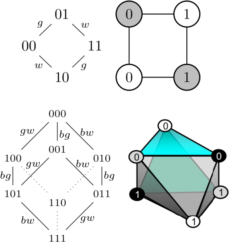
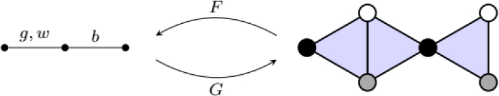
Binary Input Model. Each agent gets an input value from the set {0,1}. Each agent knows its own input value, but doesn’t know which value has been received by the other agents. The figure below from [25] shows the binary input simplicial model and its associated Kripke model for two agents, and for comparison also for three agents (although we will not use it in this paper). Notice that every possible combination of 0’s and 1’s is a possible world.
In the Kripke model, the agents are called b, g, w, and the labeling L of the possible worlds is represented as a sequence of values, e.g., 101, representing the values chosen by the agents b, g, w (in that order). In the 3-agents case, the labels of the dotted edges have been omitted to avoid overloading the picture, as well as other edges that can be deduced by transitivity.
In the simplicial model, agents are represented as colors (black, grey, and white).
The labeling ℓ is represented as a single value in a vertex, e.g., “1” in a grey vertex means that agent g has chosen value 1.
The possible worlds correspond to edges in the 2-agents case, and triangles in the 3-agents case. Note that the simplicial model depicted on the right, with three agents, is out of the scope of this paper.
Indeed, here we only work with two agents, so that the simplicial complex is nothing more than a graph.
Semantics. The definition below mimics the usual semantics of formulas in Kripke models, reformulated here in terms of simplicial models:
Definition 3.1 We define the satisfaction relation M,X⊨ϕ determining when a formula φ is true in some epistemic state (M,X). Let M=C,χ,ℓ> be a simplicial model, X∈ℱ(C) an edge of C and φ∈K:
| M,X⊨p |
iff |
p∈ℓ(X), |
| M,X⊨¬φ |
iff |
M,X⊨φ, |
| M,X⊨φ∧v |
iff |
M,X⊨φ∧M,X⊨v, |
| M,X⊨Kaφ |
iff |
∀Y∈ℱ(C),a∈χ(X∩Y), |
| |
|
⇒M,Y⊨φ. |
Group Knowledge. For a formula φ, we write Eφ=Kgφ∧Kwφ for the group knowledge of φ among the agents {g,w}. Let Ek denote k nested E operators. An edge path is a sequence of (not necessarily distinct) edges, such that each two consecutive edges in the sequence intersect in a vertex. For an edge X let be the set of edges reachable from X by an edge path of at most k edges. Thus, N1(X)={X}, denoted by N(X). Also, N2(X) is equal to X together with the edges that intersect X, and in general Nk(X)=N(Nk−1(X)).
Lemma 3.1 For a simplicial model M, edge X, and any φ∈ℒK, we have that M,X⊨Ekφ, iff M,Y⊨Eφ for every Y∈Nk(X).
The figure below is an illustration of the cases k=1,2. It shows that M,X⊨Eφ states that φ should hold in X and in its two neighboring edges, namely, in the edges that belong to N2(X), and analogously for k=2.
Morphisms Between Models Let C and D be two graphs. A simplicial mapfn f:C→D maps the vertices of C to vertices of D, such that if X is an edge of C, f(X) is an edge of D. A chromatic simplicial map between two chromatic graphs is a simplicial map that preserves colors, i.e. χ(f(v))=χ(v) for all v.
Lemma 3.2 Let f:C→D be a simplicial map. If C′ is a connected subgraph of C then f(C′) is a connected subgraph of D.
A morphism of simplicial models f:M→M′ is a chromatic simplicial map that preserves the labeling: ℓ′(f(v))=ℓ(v). The next theorem from [25] states that morphisms of simplicial models cannot “gain knowledge”.
Lemma 3.3 (Knowledge Gain) Consider simplicial models M=C,χ,ℓ> and M′=C′,χ′,ℓ′>, and a morphism f:M→M′. Let X∈ℱ(C) be an edge of M,a an agent, and φ∈ℒCK a positive formula, i.e. which does not contain negations except, possibly, in front of atomic propositions. Then, M′,f(X)⊨φ implies M,X⊨φ.
3.2 Dynamic Epistemic Logic Basic Notions
Dynamic epistemic logic (DEL) is the study of modal logics of model change [4, 13]. A modal logic studied in DEL is obtained by using action models [3]. An action can be thought of as an announcement made by the environment (not necessarily public). An action model describes all the possible actions that might happen, as well as how they affect the different agents. The product-update operation takes an epistemic model M and an action model A, and creates a new model M[A] that describes all the new possible worlds after an action from A has occurred in M. This classic version is described in Appendix 10, here we present the simplicial model version [25, 26].
Action Models A simplicial action model T,χ,pre> consists of a chromatic graph T,χ>, where the edges ℱ(T) represent communicative actions, and pre assigns to each edge X∈ℱ(T) a precondition formula pre(X) in K.
Given two chromatic graphs C and T of dimension n, the Cartesian product C×T is the following chromatic graph. Its vertices are of the form (u,v) with u∈V(C) and v∈V(T) such that χ(u)=χ(v); the color of (u,v) is χ((u,v))=χ(u)=χ(v). Its edges are of the form X×Y={(u0,v0),…,(uk,vk)} where X={u0,…,uk}∈C, Y={v0,…,vk}∈T and χ(ui)=χ(vi).
Let M=C,χ,ℓ> be a simplicial model, and A=T,χ,pre> be a simplicial action model. The product update simplicial model M[A]=C[A],χ[A],ℓ[A]> is a simplicial model whose underlying graph is a subgraph of the Cartesian product C×T, induced by all the edges of the form X×Y such that pre(Y) holds in X, i.e., M,X⊨pre(Y). The valuation ℓ:V(C[A])→  (AP) at a pair (u,v) is just as it was at u:ℓ[A]((u,v))=ℓ(u).
4 An Action Model for Dynamic Networks
Distributed Computing Model For two processes, the model G where approximate agreement is solvable, but not consensus, is unique: It consists of the three digraphs Gg, Gw, Ggw on two vertices, g, w, one with the antiparallel arrows, and the other two with an arrow from one vertex to the other, meaning that either both messages arrive, or only one. It is easy to see that in any submodel of G consensus can be solved (if it has at least one arrow). The model G is equivalent to several message passing and shared memory models that have been previously considered, see e.g. [1, 18].
Each agent has some input value, and they communicate r rounds. In each round an agent sends a message to the other agent, and the message arrives by the end of the round, or not at all. Which messages arrive depends on which graph from G is selected (it is convenient to assume that each vertex of a graph of G has a loop; an agent learns its own messages. But we do not draw the loops in the figures). In every round, any of the three graphs in G can be selected.
Input Model An input model, ℐ, represents all the possible input values. To illustrate the ideas, we use the input simplicial model of Section 3.1 where two agents A={g,w} each has an input value from the set {0,1}.
Actions An actionfn t∈T^ is given by b0, b1, c, where c is a sequence of r digraphs from G and b0,b1∈{0,1} are binary values, representing the inputs of both processes. Such an action is written cb0b1. The precondition pre(cb0b1) of this action is a formula expressing the fact that the inputs of the agents g, w are respectively b0, b1. Formally, if inputax denotes the atomic proposition expressing that agent a has input value x, then pre(xb0b1)=inputgb0∧inputwb1.
Distributed Algorithm An action t=cb0b1 includes all the information about the inputs and message deliveries of an execution, but not about the actual algorithm being executed by the agents. Namely, an algorithm specifies the contents of messages sent in each round, and the state transition of each agent. Each agent starts in an initial state, determined by its input value. At the end of a round, each agent changes to a new state following a deterministic transition function, based on its current state, and on the message received. The new state of the agent determines the message sent in the new round. The local state of agent a at the end of execution t is denoted viewa(t).
For example, consider the execution c=Gw,Ggw,Gg, meaning that in the first round only w receives a message; in the second round both processes receive a message; and in the last round only g receives a message. Picking b0=0 and b1=1 gives us the action c01, where g starts with value 0 and w starts with value 1. This is independent of the algorithm. In the algorithm of Figure 1, local states are simply the value of variable ℓ, so this action leads to the local states viewg(c01)=4/27 and vieww(c01)=3/27. In the one-bit algorithm of Figure 2, the local states are the views, so this action leads to the local states viewg(c01)= ⊥01 and vieww(c01)=00⊥.
Indistinguishability The indistinguishability relation t~at′ is a function of both the actions t, t′ and the algorithm. It is defined as t~at′ iff viewa(t)=viewa(t′).
Action Model For a given algorithm, we can reformulate the indistinguishability relation as a simplicial action model T,χ,pre> where T,χ> is a chromatic graph whose vertices are V(T)={a,viewa(cb0b1)>|a∈A,cb0b1∈T^} and whose edges are of the form, for each action cb0b1∈T^, X={<b,vieww(cb0b1)>,<g,viewg(cb0b1)>}. The precondition of such a facet is pre(X)=inputwb0∧inputgb1.
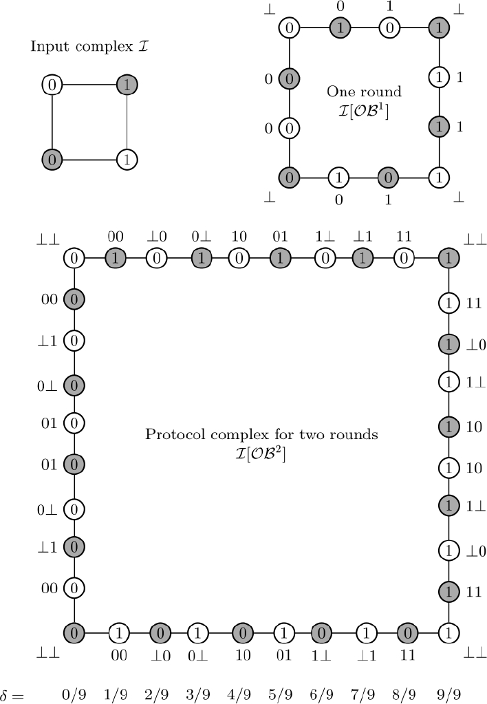
We write Ar for the simplicial action model of the r-round averaging algorithm of Figure 1, and Pℬr for the action model of the r-round one-bit algorithm of Figure 2. We also write DNr for a generic r-round dynamic network action model over an unspecified algorithm. The action models Pℬ1 and Pℬ2 are depicted in Figure 4 (as we mention below, DNr and ℐ[DNr] are always isomorphic). For r=1, each of the four input edges has been subdivided into 3 “smaller” edges: one for each possible graph of G. The colors white, grey, of the vertices correspond respectively to agents w, g. The view of each vertex is written next to it. The precondition of the three top edges is true exactly in the top edge of the input model ℐ on the left, and similarly for the other sides of the square. For r=2, the situation is similar except that each edge of ℐ is subdivided into 32=9 edges.
Perhaps surprisingly, the product update models ℐ[Ar] and ℐ[Pℬr] are isomorphic, meaning that both algorithms from Figures 1 and 2 acquire the same knowledge. They both subdivide each edge of the input complex into exactly 3r edges, thus they are both also isomorphic to the well-known full-information protocol complex.
Theorem 4.1 Let ℐ be the binary input model for two processes. For any number of rounds r, the product update models ℐ[Ar] andℐ[Pℬr] are isomorphic.
Properties about the Action Model One last thing to notice about this construction is that, when we compute the product update model ℐ[DNr], we obtain a simplicial model whose underlying graph is the same as the one of DNr. So, starting from the input model ℐ, the effect of applying DNr is to subdivide each edge of the input (the same thing happens for any other input model). Remarkably, the topology of the input graph is preserved. And in fact, there is a rate of subdivision speed, determined by the constant 1/3. These are the two basic properties that we will need in the analysis of approximate agreement (known in several specific contexts e.g. [12, 18]). Remarkably, they hold for any algorithm, not only full information algorithms.
Theorem 4.2 For any algorithm for two agents, if the input model ℐ is connected, then the product update model ℐ[DNr] is connected. Furthermore, each edge is subdivided into at most 3r edges.
We have seen that the two properties mentioned in this theorem hold for a full information algorithm. It is not hard to see that they hold for any algorithm, since the indistinguishability relation of a non-full information algorithm is a coarsening of the full information indistinguishability algorithm.
5 Tasks
The action models of the previous section, Ar and Pℬr, describe how the knowledge of the processes evolve when we execute a specific algorithm. Both of those algorithms are solving the same distributed task, namely, approximate agreement. In this section, we introduce the notion of task, which is an abstract specification of the goal that we are trying to solve, independently of the particular algorithm used to solve it. Informally, a task specifies for each possible input configuration, what are the possible output values that the agents may decide. This is once again formalized using the notion of action model; however, in the case of tasks, the actions do not correspond to communicative events, but to decisions taken by the processes. Tasks have been studied since early on in distributed computability [5]. The DEL semantics that we use here was first introduced in [25].
Consider a simplicial model ℐ=I,χ,ℓ> called the initial simplicial model. Each edge of I, with its labeling ℓ, represents a possible initial configuration. We fix ℐ, the binary inputs model of Section 3.1.
A task for ℐ is a simplicial action model T= <T,χ,pre> for agents A, where each edge is of the form X={<w,dw>,<g,dg}. The values dw, dg are taken from an arbitrary domain of output values. Each such X has a precondition that is true in one or more facets of ℐ, interpreted as “if the input configuration is a facet in which pre(X) holds, and every agent a∈A decides on the value da, then this is a valid execution”.
5.1 Semantics of Task Solvability
Given the simplicial input model ℐ and a communication model A such as DNr, we get the simplicial protocol model ℐ[A], that represents the knowledge gained by the agents after executing A. To solve a task T, each agent, based on its own knowledge, should produce an output value, such that the edge with the output values corresponds to an edge of T, respecting the preconditions of the task.
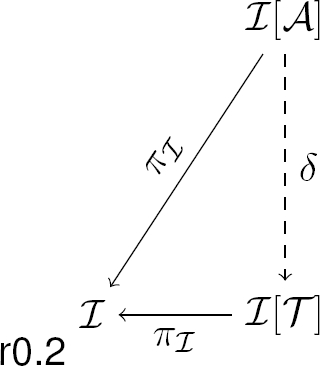
The following gives a formal epistemic logic semantics to task solvability. Recall that a morphism δ of simplicial models is a chromatic simplicial map that preserves the labeling: ℓ′(δ(v))=ℓ(v). Also recall that the product update model ℐ[A] is a subgraph of the Cartesian product ℐ×A, whose vertices are of the form (i,ac) with i a vertex of ℐ and ac a vertex of A. We write πℐ for the first projection on ℐ, which is a morphism of simplicial models.
Definition 5.1 A task T is solvable using the algorithm A if there exists a morphism δ:ℐ[A]→ℐ[T] such that πI∘δ=πI, i.e., the diagram of simplicial complexes below commutes:
The justification for this definition is the following. An edge X in ℐ[A] corresponds to a pair (i,ac), where i is an edge of ℐ representing input value assignments to the agents, and ac is an edge of A codifying the communication exchanges that took place. The morphism δ takes X to an edge δ(X)=(i,dec) of ℐ[T], where dec is the edge of T defining the set of decision values that the agents will choose in X. Moreover, pre(dec) holds in i, meaning that dec corresponds to valid decision values for input i. The commutativity of the diagram expresses the fact that both X and δ(X) correspond to the same input assignment i. Now consider a single vertex v∈X with χ(v)=a∈A. Then, agent a decides its value solely according to its knowledge in ℐ[A]: if another edge X′ contains v, then δ(v)∈δ(X)∩δ(X′), meaning that a has to decide on the same value in both edges.
Two observations about the diagram. First, by Lemma 3.3, we know that the knowledge of each agent can only decrease (or stay constant) along the δ arrow. So, any (positive) formula which is known in ℐ[T] should already be known in ℐ[A]. In other words, the goal of the agents is to improve knowledge through communication, by going from ℐ to ℐ[A], in order to match the knowledge required by ℐ[T]. Second, the possibility of solving a task depends on the existence of a certain simplicial map from the graph of ℐ[A] to the graph of ℐ[T]. We have already seen the appearance of a topological property in Theorem 4.2. Here again topology appears: a simplicial map is the discrete equivalent of a continuous map, thus connectivity is preserved by simplicial maps (Lemma 3.2); hence the topological nature of task solvability.
5.2 Approximate Agreement
Recall that in the approximate agreement problem agents are required to decide on values which are close to each other. We have seen in Section 2 that no matter how close to each other one requires the agents to decide, this task is solvable in the DNr model, taking a sufficiently large r. Many versions of this task have been considered e.g. [10]. We present here the version of [25], for two agents g and w, which is at the core of previously considered situations.
The input complex is the binary input complex for two agents of Section 3.1: so, every possible combination of 0 and 1 can be assigned to the two agents. Their goal will be to output real values in the interval [0,1], such that: (i) if their input is the same, they both decide the same output, and (ii) if their input is different, they both decide on values dg and dw such that |dg−dw|≤ε, for some fixed parameter ε∈[0,1]. A discrete version of this task is N-approximate agreement, where the output values are only allowed to be of the form k/N for 0≤k≤N. The two decision values should be within 1/N of each other: |dg−dw|≤1/N. And to simplify the presentation, let us assume N is odd, without loss of generality, in the sense that to solve ε-agreement, one has to select N large enough, so that 1/N≤ε.
Let ℐ= <I,χ,ℓ> be the input simplicial model for two agents with binary inputs, and T= <T,χ,pre> be the following action model. The set of vertices of T is V(T)={(a,k/N)|a∈A and 0≤k≤N}. The facets of T are edges Xk,k′={(g,k/N),(w,k′/N)} with |k−k′|≤1. The color of a vertex is χ(a,k/N)=a. The precondition pre(X0,0) is true in the worlds 00, 01 and 10 of ℐ; the precondition pre(XN,N) is true in the worlds 11, 01 and 10; and all the other preconditions pre(Xk,k′) are true in the worlds 01 and 10. In the figure below are the input model ℐ (left) and the action model T (right), for N=5:
The product update simplicial model ℐ[T] is depicted in the next figure, for N=5.
The numbers depicted in the nodes are the atomic propositions describing the input values from ℐ. The decision values (of the form k/5) are implicit, the first column of nodes corresponds to the decision value 0, the second column is decision value 1/5, and so on.
6 Approximate Agreement Solvability
The world X on the figure is the one with the most knowledge in the following sense. We write ϕ01 for the formula expressing that the two inputs are different. Recall (Section 3.1) that Eϕ=Kgϕ∧Kwϕ for the group knowledge of ϕ among the agents {g,w}. Then, we have ℐ[T],X⊨E3ϕ01. On the other hand, the world Y has less knowledge: we have ℐ[T],Y⊨E2ϕ01, but ℐ[T],Y⊨E3ϕ01.
Lemma 6.1 In the simplicial model ℐ[T] for the N-approximate agreement task, there are two worlds X, Y which satisfy the formula Ekϕ01, for k=⌈N/2⌉.
Proof. We choose the worlds in the “middle” of the model ℐ[T], as shown in the picture above. More formally, recall that the vertices of ℐ[T] are defined as tuples (a,i,d) where a is an agent, i its input value and d its decision value. The world X is defined as the edge {(g,1,⌊N/2⌋/N),(w,0,(⌊N/2⌋+1)/N)}, and Y={(w,1,⌊N/2⌋/N),(g,0,(⌊N/2⌋+1)/N)}. Checking that the formula is satisfied in these worlds simply consists in computing the length of the shortest path to one of the 00 or 11 edges on the sides (Lemma 3.1).
Solvability of Approximate Agreement We now study the solvability of approximate agreement in the r-round dynamic graph model DNr. Recall that each round subdivides each edge into three edges (Theorem 4.2). The picture below shows the input model ℐ, the model ℐ[DN] after one round, and the model ℐ[DN2] after two rounds:
Lemma 6.2 In the r-round model ℐ[DNr], there is no world X such that ℐ[DNr],X⊨Ekϕ01, for k=⌈3r/2⌉.
Proof. After r rounds each of the four edges of the input model ℐ has been subdivided into 3r edges. Thus, every world is at a distance at most k−1 from the nearest world with inputs 00 or 11.
Putting the two lemmas together, we get the following result:
Theorem 6.1 The N-approximate agreement task is not solvable in the r-round model ℐ[DNr], when N≥3r+1.
Proof. Assume for contradiction that the task is solvable. Then, we would have a map δ:ℐ[DNr]→ℐ[T]. Our goal is to find a contradiction using Lemma 3.3. To achieve this, we should find a formula ϕ and a world Z of ℐ[DNr], such that ϕ is false in Z but true in δ(Z) . We choose the formula ϕ:=Ekϕ01 for k=⌈N/2⌉. Since N≥3r+1 implies ⌈N/2⌉≥⌈3r/2⌉, we know by Lemma 6.2 that this formula is false in every world Z of ℐ[DNr]. All that remains to do is prove that there exists a world of ℐ[T], which is in the image of δ, and where the formula ϕ is true.
Since ℐ[DNr] is connected, its image δ(ℐ[DNr]) is connected (by Lemma 3.2). Moreover, the world 00 and the world 11 of ℐ[T] must both be in the image of δ, because of the commutative diagram of Definition 5.1. By connectedness, at least one of the middle worlds X, Y of Lemma 6.1 must belong to the image of δ. By Lemma 6.1, this world satisfies ϕ, which concludes the proof.
Conversely, we have seen in Section 2 that N-approximate agreement is solvable in r rounds whenever N=3r. The proof of the above theorem sheds light on the required knowledge to solve approximate agreement: while consensus is about reaching common knowledge, approximate agreement is about reaching some finite level of nested knowledge.
7 Approximate Agreement Algorithms
Here we provide additional details about the correctness of the algorithms described in Section 2. Recall that N=3k, agents start with values in 0, 1, and they have to decide values at most 1/N apart, unless their inputs are equal, in which case their outputs should be equal to their inputs. First we show that the algorithm in Figure 1 solves N-approximate agreement in k rounds.
Theorem 7.1 The algorithm Averaging Approximate Agreement is correct.
Proof. Let mep be the initial value of agent p.
For k=1, suppose w.l.g. that the message from g arrives, then the final value of agent w is dw=(mew+2meg)/3. If both messages arrives then dw=(meg+2mew)/3 so |dw−dg|=|(2meg−meg+mew−2mew)/3|=|(meg−mew)/3|≤1/3. If just one message arrives then dg=meg, so |dw−dg|=|(mew+2meg−3meg)/3|=|(mew−meg)/3|≤1/3. Let dpk be the final value of agent p after k rounds, and suppose that |dwk−dgk|K,1/3k for some k, then, if message from g arrives in round k+1 (w.l.g.), dwk+1=(dwk+2dgk)/3. The rest of the proof is analogous to induction base, analysing both cases whether message from w gets lost or not.
To prove the correctness of the One-Bit Messages algorithm of Figure 2, we rely on Theorem 4.1. So let us prove it first:
Theorem 4.1. Let ℐ be the binary input model for two processes. For any number of rounds r, the product update models ℐ[Ar] and ℐ[Pℬr] are isomorphic. Proof. Recall that ℐ[Ar] is the product update model for r-rounds of the Averaging algorithm in Figure 1, and ℐ[Pℬr] is the product update model for r-rounds of the One-Bit algorithm of Figure 2.
It is well known that ℐ[Ar] is isomorphic to the full-information protocol complex, which subdivides each edge of the input into 3k edges, preserving the topology. Thus, we show that ℐ[Pℬr] does the same thing.
We proceed by induction on r. For the one-round algorithm, ℐ[Pℬ1] is depicted in Figure 4, and indeed each edge of the input complex has been subdivided into three.
Let us now assume that ℐ[Pℬr] is indeed isomorphic to ℐ[Ar], i.e., that each edge of ℐ has been subdivided in 3k small edges.
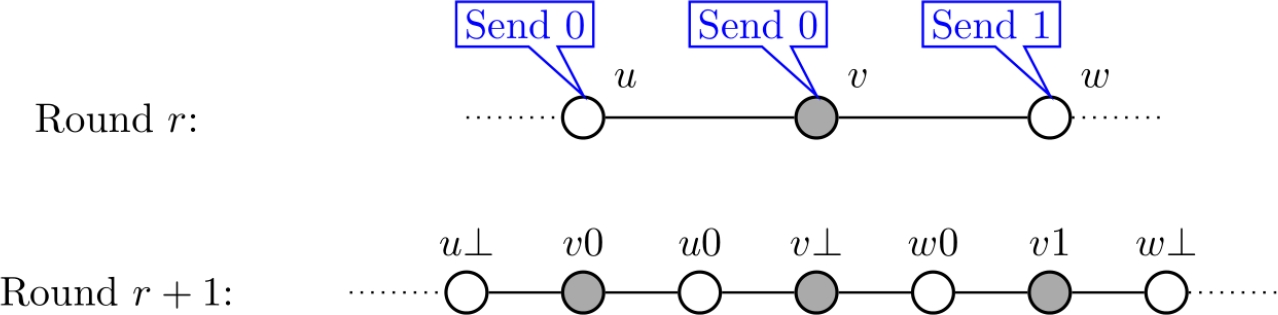
Consider an arbitrary vertex of ℐ[Pℬr] (a grey vertex w.l.o.g.), of the form <g,viewg(t)> for some action t=cb0,b1. Let us write v=viewg(t) for the view of this vertex.
Moreover, let us assume that the two neighbors of this vertex, with views u and w, are about to send two distinct messages, 0 and 1 respectively. (One can check that this property is true everywhere in
ℐ[Pℬ1]: every vertex has neighbors that will send different messages in the next round.)
After one more round of the one-bit algorithm, we obtain six edges in ℐ[Pℬr+1] as depicted below (we assume w.l.o.g. that the grey vertex sends the message “0”; the same picture can be drawn with a 1 instead). Moreover, we can check that the five vertices in the middle at round r+1 still have the inductive property that both neighbors will send a different message at the next round.
This local reasoning can be done around each node of ℐ[Pℬr]. Thus, every edge is subdivided into 3, which concludes our proof.
Now we can show that the algorithm in Figure 2 solves N-approximate agreement in k rounds.
Theorem 7.2 The algorithm One-Bit Messages Approximate Agreement is correct.
Proof. Since ℐ[Pℬr] is isomorphic to ℐ[Ar], and we have shown in Theorem 7.1 that ℐ[Ar] solves 3r-approximate agreement, we know that the One-Bit algorithm can solve approximate agreement as long as we choose the right decision function δ.
This is precisely what the algorithm from Figure 3 does: δ(ℓ,view) simulates the Average Approximate Agreement algorithm via the isomorphism exhibited in Theorem 4.1. A detailed proof of correctness can be found in [12].
8 Simplicial Models and Epistemic Logic
Here we include generalized notions for any number of agents from section 3.
Generalizing graphs to complexes Given a set V, a simplicial complex C is a family of non-empty finite subsets of V such that for all X∈C, Y⊆X implies Y∈C. We say Y is a face of X. Elements of V (identified with singletons) are called vertices. Elements of C are simplexes, and those which are maximal w.r.t. inclusion are facets. The set of vertices of C is noted V(C), and the set of facets ℱ(C). The dimension of a simplex X∈C is |X|−1, and a simplex of dimension n is called an n-simplex. A simplicial complex C is pure if all its facets are of the same dimension, n. In this case, we say C is of dimension n. A graph without isolated vertices is a pure sumplicial complex of dimension 1. Given the set A of agents (that we will represent as colors), a chromatic simplicial complex <C,χ> consists of a simplicial complex C and a coloring map χ:V(C)→A, such that for all X∈C, all the vertices of X have distinct colors.
Simplicial Maps Let C and D be two simplicial complexes. A simplicial map f:C→D maps the vertices of C to vertices of D, such that if X is a simplex of C, f(X) is a simplex of D. A chromatic simplicial map between two chromatic simplicial complexes is a simplicial map that preserves colors. Let SA be the category of pure chromatic simplicial complexes on A, with chromatic simplicial maps for morphisms.
Equivalence with Epistemic Logic A Kripke frame M= <S,~> over a set A of agents consists of a set of states S and a family of equivalence relations on S, written ~a for every a∈A. Two states u, v∈S such that u~a v are said to be indistinguishable by a. A Kripke frame is proper if any two states can be distinguished by at least one agent. Notice that being proper means that the intersection of all equivalence relations ~a is the identity; this may reveal interesting parallels with distributed knowledge (a formula that is true in all states in the intersection relation), see e.g. [24]. Let M= <S,~> and N= <T,~′> be two Kripke frames. A morphism from M to N is a function f from S to T such that for all u, v∈S, for all a∈A, u~a v implies f(u)~′a f(v). We write KA for the category of proper Kripke frames, with morphisms of Kripke frames as arrows.
The following theorem states that we can canonically associate a proper Kripke frame with a pure chromatic simplicial complex, and vice versa. In fact, this correspondence extends to morphisms, and thus we have an equivalence of categories, meaning that the two structures contain the same information.
Theorem 8.1 ([25]) SA and KA are equivalent categories.
Example 8.1 ([25]) The picture below shows a Kripke frame (left) and its associated chromatic simplicial complex (right). The three agents, named b, g, w, are represented as colors black, grey and white on the vertices of the simplicial complex. The three worlds of the Kripke frame correspond to the three triangles (i.e., 1-dimensional simplexes) of the simplicial complex. The two worlds indistinguishable by agent b, are glued along their black vertex; the two worlds indistinguishable by agents g and w are glued along the grey-and-white edge.
Simplicial Models Let be some countable set of values, A be a finite set of agents and AP={pa,x|a∈A,x∈V} be the set of atomic propositions. Intuitively, pa,x is true if agent a holds the value x. We write APa for the atomic propositions concerning agent a. A simplicial model M= <C,χ,ℓ> consists of a chromatic simplicial complex <C,χ>, and a labeling ℓ:V(C)→P(AP) that associates with each vertex v∈V(C) a set of atomic propositions concerning agent χ(v), i.e., such that ℓ(v)⊆APχ(v). Given a simplex X∈C, we write ℓ(X)=∪i=0nℓ(vi). A morphism of simplicial models f:M→M′ is a chromatic simplicial map that preserves the labeling: ℓ′(f(v))=ℓ(v). We denote by SℳA,AP the category of simplicial models over the set of agents A and atomic propositions AP.
Equivalence with Epistemic Logic A Kripke model M= <S,~,L> consists of a Kripke frame <S,~> and a function L:S→P(AP). Intuitively, L(s) is the set of atomic propositions that are true in the state s. A Kripke model is proper if the underlying Kripke frame is proper. A Kripke model is local if for every agent a∈A, s~as′ implies L(s)∩APa=L(s′)∩APa, i.e., an agent always knows its own values. Let M= <S,~,L> and M′= <S′,~′,L′> be two Kripke models on the same set AP. A morphism of Kripke models f:M→M′ is a morphism of the underlying Kripke frames such that L′(f(s))=L(s) for every state s in S. We write KℳA,AP for the category of local proper Kripke models.
[[25]] Given a simplicial model M and a facet X,M,X⊨φ iff F(M),X⊨Kφ. Conversely, given a local proper Kripke model N and state s,N,s⊨Kφ iff G(N),G(s)⊨φ, where G(s) is the facet {v0s,…,vns} of G(N).
We can now extend Theorem 8.1 to an equivalence between simplicial models and Kripke models.
Theorem 8.2 ([25]) SℳA,AP and KℳA,AP are equivalent categories.
9 Knowledge in Simplicial Models
Here we include additional details about group knowledge and knowledge gain from subsection 3.1.
Lemma 3.1 For a simplicial model M and edge X, we have that M,X⊨Ekϕ, iff M,Y⊨Eφ for every Y∈Nk(X).
Proof. For k=1 the proof is immediate.
Let k such that M,X⊨Ekϕ iff M,Y⊨Eϕ for every Y∈Nk(X). Then M,X⊨Ek(Eϕ) iff M,Z⊨E2ϕ for every Z∈Nk(X). Finally M,Y⊨Eϕ for every Y∈N2(Z) such that Z∈Nk(X), i.e. Y∈Nk+1(X) (since Nk+1(X)=N(Nk(X))).
Lemma 3.3 Consider simplicial models M= <C,χ,ℓ> and M′= <C′,χ′,ℓ′>, and a morphism f:M→M′. Let X∈ℱ(C) be an edge of M, a an agent, and φ∈ℒCK a positive formula, i.e. which does not contain negations except, possibly, in front of atomic propositions. Then, M′,f(X)⊨φ implies M,X⊨φ.
Proof. Suppose that ϕ is atomic, then M′,f(X)⊨ϕ iff ϕ∈l(f(X))=l(X), so M,X⊨ϕ.
If ϕ=¬p for some atomic p then M′,f(X)⊨p, so p∉l(f(X))=l(X), therefore M,X⊨p.
If ϕ=ψ∧θ for some formulas ψ and θ as depicted above, then M′,f(X)⊨ψ and M′,f(X)⊨θ.
Therefore M,X⊨ψ∧θ.
If ϕ=Ka(ψ) with ψ being a formula like depicted above, let Y∈ℱ(M) such that a∈χ(Y∩X), then a∈χ(f(Y)∩f(X)) so M′,f(Y)⊨ψ and therefore M,Y⊨ψ, implying that M,X⊨ϕ.
Finally, every possitive formula can be seen as combinations of formulas like depicted above but linked with ∧. Hence, if ϕ=∧i∈ψi then for all i∈, M′,f(X)⊨ψi so that M,X⊨ψi. Finally, M,X⊨∧i∈ψi.
10 Dynamic Epistemic Logic
Here we presents the classic version of DEL.
An action model is a structure <T,~,pre>, where T is a domain of action points, such that for each a∈A, ~a is an equivalence relation on T , and pre:T→K is a function that assigns a precondition formula pre(t) to each t∈T. Let M= <S,~,L> be a Kripke model and A = <T,~,pre> be an action model. The product update model is M[A]= <S[A],~[A],L[A]>, where each world of S[A] is a pair (s,t) with s∈S, t∈T such that pre(t) holds in s. Then, (s,t)~a[A](s′,t′) whenever it holds that s~as′ and t~at′. The valuation L[A] at a pair (s,t) is just as it was at s, i.e., L[A]((s,t))=L(s). For an initial Kripke model M, the effect of action model A is a Kripke model M[A]. Notice that if M is a local proper Kripke model and A= <T,~,pre> is a proper action model, then M[A] is proper and local.
Equivalence with Simplicial Action Models Recall from Theorem 8.2 the two functors F and G that define an equivalence of categories between simplicial models and Kripke models. We have a similar correspondence between action models and simplicial action models. On the underlying Kripke frame and simplicial complex they are the same as before; and the precondition of an action point is just copied to the corresponding facet. The following proposition says that the “classic” product update agrees with the “fully simplicial” one.
Consider a simplicial model M and simplicial action model A, and their corresponding Kripke model F(M) and action model F(A). Then, the Kripke models F(M[A]) and F(M)[F(A)] are isomorphic. The same is true for G, starting with a Kripke model M and action model A.
Proof. Particular case of theorem 8.2, since F(M[A]) is the image of F(M)[F(A)] under the functor who states equivalence.
11 Dynamic Networks and Tasks
Here we include additional details about Section 4 and 5.
Theorem 4.2 For any algorithm for two agents, the product update model M[DNr] is a graph which is connected (assuming the input model is connected). Furthermore, each edge is subdivided into at most 3r edges.
Proof.
Since underlying simplicial complex of M[DNr] is the same as the one of G(DNr), we just need to prove that G(DNr) is connected.
For r=1, let ℐ be the input model, then the function who carries any edge X of ℐ into the set {X∈ℱ(G(DNr))|M,{(b,b0),(g,b1)}⊨pre(X)} is bijective. Moreover f[ℐ]=ℱ(G(DN)) and since any edge X∈ℱ(ℐ) is such that |f(X)|=3, X splits into 3 edges in G(DN).
Now consider arbitrary edges X,Y∈ℱ(ℐ) and let Xi,Yj∈ℱ(G(DN)) subdivisions of X, Y respectively. Since ℐ is connected, exists (X,Z1,…,Zn,Y) a sequence of connected edges in ℐ. Hence, in G(DN) we have another edge path who links Xi with any subdivision of Z1, which is linked with any subdivision of Z2 and so on, until reach any subdivision of Zn, and finally Yj.
For r such that G(DNr) is connected, we can consider G(DNr) as an input model, and since G(DNr+1) is also the underlying graph of (M[DNr])[DN], the rest of the proof is analogous to induction base. Finally, since each edge is already subdivided into 3r edges in G(DNr), they are subdivided into 3(3r)=3r+1 edges in G(DNr+1).
12 Conclusions
We have considered a basic notion of approximate agreement, and a computational model for two agents, where the task is solvable for any desired level of precision. We first presented two algorithms, which solve the task for a given precision level, using the same number of communication rounds. With this concrete setting in mind, we have proceeded to give a formal semantics based on dynamic epistemic logic, both to our computational model, and to the approximate agreement task. We derived a lower bound result showing that these algorithms are optimal in the number of rounds. The lower bound is due to the impossibility of the agents gaining global knowledge about their inputs faster, and a consequence of the connectivity of the computational model’s epistemic states. Although much of these results were previously known, we have made an effort to distil the essential ingredients of several previous papers, and combined them into a unified, self-contained way, providing thus a more elementary introduction to the area, based only of graph theory, instead of higher dimensional simplicial complexes.
Acknowledgments
This work is partially supported by UNAM-PAPIIT grant IN106520 (Sergio Rajsbaum).
References
1. Attiya, H., Rajsbaum, S. (2002). The combinatorial structure of wait-free solvable tasks. SIAM J. Comput., Vol. 31, No. 4, pp. 1286–1313.
[ Links ]
2. Attiya, H., Rajsbaum, S. (2020). Indistinguishability. Commun. ACM, Vol. 63, No. 5, pp. 90–99.
[ Links ]
3. Baltag, A., Moss, L., Solecki, S. (1998). The logic of common knowledge, public announcements, and private suspicions. TARK VII, pp. 43–56.
[ Links ]
4. Baltag, A., Renne, B. (2016). Dynamic epistemic logic. In The Stanford Encyclopedia of Philosophy, see https://plato.stanford.edu/archives/win2016/entries/dynamic-epistemic/. Metaphysics Research Lab, Stanford University.
[ Links ]
5. Biran, O., Moran, S., Zaks, S. (1990). A Combinatorial Characterization of the Distributed 1-Solvable Tasks. J. Algorithms, Vol. 11, No. 3, pp. 420–440.
[ Links ]
6. Braud-Santoni, N., Dubois, S., Kaaouachi, M.-H., Petit, F. (2016). The next 700 impossibility results in time-varying graphs. Int. J. Netw. Comput., Vol. 6, pp. 27–41.
[ Links ]
7. Castañeda, A., Fraigniaud, P., Paz, A., Rajsbaum, S., Roy, M., Travers, C. (2019). A topological perspective on distributed network algorithms. Censor-Hillel, K., Flammini, M., editors, Structural Information and Communication Complexity - 26th International Colloquium, SIROCCO 2019, L’Aquila, Italy, July 1-4, 2019, Proceedings, volume 11639 of Lecture Notes in Computer Science, Springer, pp. 3–18.
[ Links ]
8. Casteigts, A., Flocchini, P., Quattrociocchi, W., Santoro, N. (2011). Time-varying graphs and dynamic networks. Frey, H., Li, X., Ruehrup, S., editors, Ad-hoc, Mobile, and Wireless Networks, Springer Berlin Heidelberg, Berlin, Heidelberg, pp. 346–359.
[ Links ]
9. Charron-Bost, B., Függer, M., Nowak, T. (2015). Approximate consensus in highly dynamic networks: The role of averaging algorithms. Halldórsson, M. M., Iwama, K., Kobayashi, N., Speckmann, B., editors, Int. Colloquium on Automata, Languages, and Programming (ICALP), number 9135 in Lecture Notes in Computer Science, Springer Berlin Heidelberg, Berlin, Heidelberg, pp. 528–539.
[ Links ]
10. Charron-Bost, B., Függer, M., Nowak, T. (2016). Fast, Robust, Quantizable Approximate Consensus. Chatzigiannakis, I., Mitzenmacher, M., Rabani, Y., Sangiorgi, D., editors, 43rd International Colloquium on Automata, Languages, and Programming (ICALP 2016), volume 55 of Leibniz International Proceedings in Informatics (LIPIcs), Schloss Dagstuhl–Leibniz-Zentrum fuer Informatik, Dagstuhl, Germany, pp. 137:1–137:14.
[ Links ]
11. Coulouma, É., Godard, E., Peters, J. G. (2015). A characterization of oblivious message adversaries for which consensus is solvable. Theor. Comput. Sci., Vol. 584, pp. 80–90.
[ Links ]
12. Delporte-Gallet, C., Fauconnier, H., Rajsbaum, S. (2020). Communication complexity of wait-free computability in dynamic networks. Richa, A. W., Scheideler, C., editors, Structural Information and Communication Complexity (SIROCCO), number 12156 in LNCS, Springer International Publishing, Cham, pp. 291–309.
[ Links ]
13. Ditmarsch, H. v., van der Hoek, W., Kooi, B. (2007). Dynamic Epistemic Logic. Springer.
[ Links ]
14. Dolev, D., Lynch, N. A., Pinter, S. S., Stark, E. W., Weihl, W. E. (1986). Reaching approximate agreement in the presence of faults. J. ACM, Vol. 33, No. 3, pp. 499–516.
[ Links ]
15. Fischer, M., Lynch, N. A., Paterson, M. S. (1985). Impossibility Of Distributed Commit With One Faulty Process. Journal of the ACM, Vol. 32, No. 2, pp. 374–382.
[ Links ]
16. Függer, M., Nowak, T., Schwarz, M. (2018). Tight bounds for asymptotic and approximate consensus. Newport, C., Keidar, I., editors, Proceedings of the 2018 ACM Symposium on Principles of Distributed Computing, PODC 2018, Egham, United Kingdom, July 23-27, 2018, ACM, pp. 325–334.
[ Links ]
17. Goubault, É., Lazić, M., Ledent, J., Rajsbaum, S. (2019). A dynamic epistemic logic analysis of the equality negation task. Dynamic Logic. New Trends and Applications - Second International Workshop, DaĹı 2019, Proceedings, pp. 53–70.
[ Links ]
18. Herlihy, M., Kozlov, D., Rajsbaum, S. (2013). Distributed Computing Through Combinatorial Topology. Elsevier-Morgan Kaufmann.
[ Links ]
19. Herlihy, M., Rajsbaum, S., Raynal, M., Stainer, J. (2017). From wait-free to arbitrary concurrent solo executions in colorless distributed computing. Theor. Comput. Sci., Vol. 683, pp. 1–21.
[ Links ]
20. Hoest, G., Shavit, N. (2006). Towards a topological characterization of asynchronous complexity. SIAM J. Comput., Vol. 36, No. 2, pp. 457–497.
[ Links ]
21. Kuhn, F., Oshman, R. (2011). Dynamic networks: models and algorithms. SIGACT News, Vol. 42, No. 1, pp. 82–96.
[ Links ]
22. Loui, M. C., Abu-Amara, H. H. (1987). Memory requirements for agreement among unreliable asynchronous processes. volume 4 of Advances in Computing Res., JAI press, pp. 163–183.
[ Links ]
23. Moses, Y., Rajsbaum, S. (2002). A layered analysis of consensus. SIAM J. Comput., Vol. 31, No. 4, pp. 989–1021.
[ Links ]
24. Fagin, R., Moses, Y., Halpern, J.Y., Vardi, M. (1995). Reasoning About Knowledge. MIT Press.
[ Links ]
25. Goubault, Éric, Ledent, J., Rajsbaum, S. (2020). A simplicial complex model for dynamic epistemic logic to study distributed task computability. Information and Computation, pp. 104597. In print, a preliminary version appeared in Proc. of GandALF 2018.
[ Links ]
26. van Ditmarsch, H., Goubault, E., Ledent, J., Rajsbaum, S. (2020). Knowledge and simplicial complexes. arXiv e-prints. To appear in the journal Information and Computation, Elsevier.
[ Links ]
27. Winkler, K., Schmid, U. (2019). An overview of recent results for consensus in directed dynamic networks. Bull. EATCS, Vol. 128.
[ Links ]


 nueva página del texto (beta)
 Inglés (pdf)
 Artículo en XML
 Referencias del artículo
 Enviar artículo por email
 Citado por SciELO
  Similares en
SciELO
Similares en
SciELO 
 Permalink