


 nova página do texto(beta)
 Inglês (pdf)
 Artigo em XML
 Referências do artigo
 Enviar este artigo por email
 Citado por SciELO
  Similares em
SciELO
Similares em
SciELO 
 Permalink
1 Introduction
To generate an orthomosaic (orthophotography), aerial-photogrammetry techniques are used. Photogrammetry is a technique that determines geometric properties and spatial relations of the terrain from aerial photographic images [3]. It is a very complex process in which the main objective is to convert two-dimensional data (flat images) into cartographic/three-dimensional data. This technique allows us to obtain the geometric properties of a surface based on information obtained from several images with redundant information. It is this repeated structure that allows the extraction of the object’s structure through the overlap among consecutive images.
The pairing of a set of overlapping images that are joined in a single image produces an orthophotography. Orthophotography allows us to have current visual knowledge of an area of interest, with validity similar to that of a cartographic plane. Nevertheless, the resolution of the orthophoto needs to be as high as possible. For this, it is necessary to use a photogrammetry software that processes aerial images to generate 3D reconstructions or orthophotos. The software searches correspondences between images and determines the correct which are its probable positions, based on the different points of view of the same element, in a process called stitching. Commercial software offers different photogrammetry services, some base on geometry and pixel values of the images.
The current capabilities of photogrammetry and machine learning techniques have been integrated to revolutionize current workflows and allow many new ones. In this work, we propose a novel methodology to generate high-resolution orthomosaics based on machine learning, whose main contributions are:
— Combining the main elements of two deep neural network models and incorporating a closed-loop feedback that optimizes the feature map, keypoints and correspondence generation process to perform stitching aerial images.
— Integrating Visual SLAM and Deep Learning techniques to improve image stitching by using a greedy algorithm widely used in Visual SLAM systems.
— Improving the image stitching processes by employing a widely used greedy algorithm and thus integrating Visual SLAM and Deep Learning techniques.
— Verifying the network’s ability to process large amounts of high-resolution images.
2 Related Work
Recent research to obtain terrain models, such as those presented in [2, 4, 12, 16, 20] perform image pairing or 3D reconstructions using deep-neural-network techniques. The resulting maps or models need to be in high-resolution (HR), therefore, the neural network must be able to work with HR aerial images. Traditional methodologies implement artificial-vision techniques and algorithms to solve problems such as SLAM and reconstruction tasks [11]. However, many of these algorithms are not optimized to work with HR images [14, 17].
To deal with this problem, some techniques and architectures have been proposed, such as the one presented in [21]. Furthermore, the problem becomes more complex when there is a large number of images involved. Nevertheless, to solve these types of problems, multiple works have been presented, ranging from image enhancement to super-resolution scaling to recover content from low-resolution (LR) images [10, 15, 26, 29].
3 Methodology
Our approach consists of two main stages. In the first stage, feature extraction and key-point correspondences are performed from high resolution input images.
These correspondences are used to stitch the input images and obtain a low-resolution orthophotography.
The second stage uses the low-resolution orthophotography obtained in the previous stage to estimate a high-resolution image. The model used in this stage is based on the SRGAN architecture and is obtained by replacing the original residual blocks with those proposed and used in stage one of the methodology.
Finally, the output of the second stage is used as input of the first stage (closed-loop feedback) to build a complete high-resolution orthomosaic. By doing so, we are able to handle a large number of high-resolution images and reconstruct large areas of land. The complete methodology is shown in Fig. 2.

Fig. 1. Results comparison. The images in the first column show the orthomosaics obtained by means of a manual reconstruction carried out by an expert. The orthomosaic obtained with our methodology shown in the second column. The last column shows the reconstruction obtained with the Pix4DMapper software

Fig. 2. The general structure of the proposed methodology consists of two stages. The first stage is in charge of matching the input images. The second stage is responsible for generating a super-resolution image from the low-resolution image obtained in the previous stage. The output of the second stage is also used as input of the first stage (feedback loop). Our methodology optimizes the orthographic generation process when working with large quantities of images. Each stage is described in subsequent sections.
3.1 Dataset
For transfer learning and fine-tuning, we created a dataset that includes 3, 000 aerial images taken at the university campus. Due to terrain conditions, safe flight height and overlapping percentage among captured images, two configurations were considered as show in Table 1.
3.2 Network Architecture
In this section we describe the proposed network architecture. Residual networks are inspired by the biological fact that some neurons connect with neurons that are not necessarily adjacent, thus skipping intermediate layers. This allows a neuron to have more connections without increasing the total number of parameters or computation complexity.
Using residual learning blocks, deeper neural networks (with more than 100 layers) can be trained due to their ability to control the vanishing gradient problem. Hence, models based on residual learning blocks are easier to optimize and ensure accuracy from a considerably increased depth. This paradigm is a basic element in many computer vision tasks.
On the other hand, a feedback methodology allows communication between the input and the output of the architecture, thus preventing information loss and improving processing times.
Therefore, we propose a neural network based on two known models. The first one is composed of 152 layers and its based on the original ResNet50 model, pre-trained with the ImageNet database. We replaced the original ReLU activation function with a parametric ReLU. We used the output of the fourth convolutional block to obtain feature maps and append a fully connected layer and an Image Retrival layer to obtain key points and correspondences of the points between each pair of images. Finally, for the geometric correction, two more layers were added: a max-pooling and a fully connected layer. With the results of these network, we employ classical computer vision techniques to obtain point correspondences and perform image stitching.
In general, a typical CNN contains several convolutional layers. These layers apply convolution between a filter and an image to generate feature maps necessary for subsequent processing. However, residual networks propose some changes as shown in Fig. 3. A typical CNN (see Fig. 3a), organizes the architecture by combining basic units such as convolution, nonlinear mapping, pooling or batch-normalization in cascade. In contrast, a residual network (see Fig. 3b), has a shortcut pathway directly connecting the input and output of a building block.

Fig. 3. Block diagram of two different CNN models. In a typical CNN model, the learning block combines basic units in cascade (see Fig. 3a). In contrast, a residual network (see Fig. 3b), has a shortcut pathway directly connecting the input and output in a building block
Mathematically, instead of approximating an underlying function
The output
However, it is easier to fit a residual mapping
Afterwards, based on the model developed by Noh et al. [19], we decided to use the cross-entropy loss function given by:
where
where the backpropagation of the output score
The second stage is based on the original SRGAN model and it generates a high-resolution image with realistic textures. We use a discriminator to distinguish the HR images and backpropagate the GAN loss. It is mostly composed of convolutional layers, batch-normalization and parameterized ReLU (PreLU). Also, the generator implements skip connections similar to ResNet. For this stage, we decided to use the same 10 residual blocks generated in stage one of our methodology and only retrain the discriminator. With this configuration, we reduced the complexity of the model and improved processing time. To train the discriminator we used the typical GAN discriminator loss.
To discriminate real HR images from super-resolution (SR) generated images, the discriminator network follows the architectural guidelines summarized by Ledig et al. [13] and Goodfellow et al.[5] by using a LeakReLU activation function
To perform fine-tuning and transfer learning we use
After twelve hours of training, we obtained a loss of

3.3 Generation of a Low-Resolution Orthomosaic
The first stage generates a stitched image from two high-resolution images. The CNN in the first stage is based on the model developed by Noh et al. [19] and is responsible for extracting dense features from the input images by using the outputs of the fourth convolutional block of the ResNet50 [8] network pretrained with the ImageNet dataset [22].
The residual blocks are designed with two convolutional layers followed by batch-normalization layers and Parametric ReLU [7] as the activation function. To be able to carry out this procedure correctly, we use transfer learning and fine-tuning using our previously generated dataset. The network’s layers are shown in figure 5a.

Fig. 5. by Noh’s work, the first stage (shown in Fig 5a.) is based on ResNet50. However, we simultaneously use two branches (each composed as shown in Fig. 5b) to extract dense features from input images.
We use image-retrieval techniques and the features obtained from the two branches to perform a feature descriptor matching for all pairs of images. We use the upper part of the max- pooling layer to establish correspondences. In Fig. 6 the feature points are marked with black circles and the correspondences between the images are marked with colored lines. Using these correspondences, image stitching is performed and the low-resultion orthomosaic is obtained.

Fig. 6. between an image pair. The output of the model in the first stage provides the correct matches between a pair of input images. The results show that the proposed methodology obtains good results even in the adverse conditions of a challenging environment, such as the university campus.
The results are acceptable and robust even in exteriors. Unfortunately, among many pairs of images, more than one pairwise-aligment ambiquity is present (see Fig. 7a).
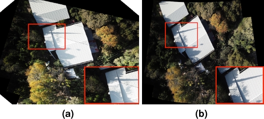
Fig. 7. of the orthomosaic. A significant improvement is shown when applying a loop closure algorithm to stitched images. Therefore, zooming in on an area of the image shows and an improvement in the stitching of the images. Visible image stitching (see Fig. 7a) and improved image stitching (see Fig. 7b)
This ambiguity cannot be eliminated using traditional computer vision techniques. Therefore, employing a pruning algorithm across this image and enforcing group consensus may be a better strategy [12]. A global-consensus restriction for loop closure has been widely adopted in SLAM [24, 18] and has shown to be effective in these tasks. For this reason, we use a Greedy Loop Closing (GLC) [12] algorithm to enforce global loop closure constraints, which eliminates ambiguities during the alignment of image pairs.
3.3.1 A Greedy Loop Closing (GLC) Algorithm
We use a directed multi-graph
In our application, each vertex
We use the correspondences obtained in the previous step to join image
where,
3.4 Generation of a High-Resolution Orthomosaic
The purpose of the second stage of our proposed methodology is to generate a high-resolution orthomosaic. To do this, we use a SRGAN inspired by the work of Wang et al. [26] and follow the architectural guidelines developed by Ledig et al. [13]. SRGAN is a generative adversarial network (GAN) for super-resolution imaging (SR) and it efficiently scales a LR image by a factor of

Fig. 8. model used to increase the scale of the input images (Fig. 8a). This model implements connections similar to those in ResNet (same blocks used in stage one) and we only retrain the discriminator as explained in section 3.2. The same upsampling block (Fig. 8b) as in the original model is used
One of the main parts of the second network is the upsampling layer used, proposed by Shi et al. [23], which increases the resolution of the input image using two blocks made up of a convolutional layer, two PixelShuffler layers and a Parametric ReLU activation function. The sub-pixel convolutional neural network aggregates the feature maps from an LR image and builds an HR image in a single step.
The periodic shuffling is fast, compared to the reduction or convolution of an HR image, because each operation is independent and thus is trivially parallelizable.
The SRGAN model receives as input and image in LR (see Fig. 9a) and is able to scale it by up to

Fig. 9. (HR) image generation. These results show that our proposal is able to generated an HR image (Fig. 9c) from a LR image (Fig. 9a). It also shows the importance of applying transfer learning and fine tuning to generate super-resolution images
The previous result (Fig. 9b) shows that fine-tuning and transfer learning must be applied, using our generated dataset, to increase the quality of the textures obtained from the SRGAN model. Once applied, we obtain the super-resolution image (Fig. 9c) which contains improved details, similar to those in the original images.
4 Experimental Results
To evaluate our proposal, we visually analyzed the qualitative results of our proposed methodology. First, we analyzed the low-resolution orthomosaic generation results (Fig. 7a), and later analyzed the result obtained after applying a loop-closure algorithm (see Fig. 7b). Also, in section 3.4, we validate the high-resolution orthmosaic generation results (see Fig. 9), which are obtained by using fine-tuning and transfer learning.
We also compared our HR orthomosaic with two other orthomosaics, the first one being a manual reconstruction done by an expert in orthophotography, and the second one being generated by a commercial software.
For testing, we selected images of different university areas. To generate the orthomosaic, we used images in
Using our proposed methodology, we were able to obtain acceptable low-resolution (Fig. 7) and a high-resolution (Fig. 9) orthomosaics. Although, each stage has been configured correctly, and both can work together to generate orthomosaics, it was observed that the first stage presents limitations when working with more than
This process improves processing times and increases the ability to work with more than 100 images. The only drawback is a decrease in the image’s resolution, which is now in HR. The results are also validated by comparing them against a manual reconstruction obtained by an expert and a reconstruction obtained using the Pix4DMapper software.
Manual reconstructions were done using high-resolution images, however, these results show inferior image quality when compared to our results. The orthomosaics obtained using commercial software (last column of Fig. 1) are in high-resolution. However, Pix4DMapper was only able to get
To analyze the similarity between the three resulting orthomosaic we use the Euclidean distance, given by equation 6 (the smaller the distance, the greater the similarity) [25, 1], which is the most commonly used image metric due to its simplicity:
Root mean square error (MSE) and peak signal-to-noise ration (PSNR) are common evaluation metrics used to compare generated high-resolution images and real images. Image-quality evaluation methods are based on comparisons using explicit numerical criteria and expressed in terms of statistical parameters and tests [9]. Peak Signal-to-Noise Ratio (PSNR) is a commonly used example.
The PSNR (measured in decibels (dB)) between two images
where
However, the ability of MSE (8) (and PSNR (7)) to differentiate perceptually relevant differences, such as high-texture detail, is very limited, as it is defined in terms of image-per-pixel differences [27, 6, 30]. Furthermore, a high PSNR value does not necessarily reflect a perceptually better HR result. The difference in perception between the original image and the supersolute image means the recovered image may not be photorealistic. We know that the objective of applying this metric is to evaluate the results obtained by an algorithm to generate super-resolution images or, in this case, the architecture of neural networks to generate high quality textures in an HR image.
The results of the evaluation of the generated orthomosaics are shown in Table 2, where we can see that the high value of PSNR corresponds with a low Euclidean distance.
Table 2 Orthomosaic comparison. This table shows the Euclidean distances as a measure of similarity, and the peak signal-to-noise ratio (PSNR) between our generated orthomosaic, a manual reconstruction obtained by an expert and an orthomosaic obtained using the Pix4DMapper software
| Orthomosaic | Euclidean distance | PSNR | Processing time | Resolution |
| Our orthomosaic | - | - | 60 mins | HR |
| Manual reconstruction | 7.294145 | 28.1705654 dB | 1500 mins | HR |
| Orthomosaic from Pix4DMapper | 20.139497 | 24.9170499 dB | 120 mins | HR |
With this, we can be certain that the results will provide high quality textures, at the pixel level, similar to those of an original image. The results, also show that the proposed methodology is better than commercial software in several aspects. Furthermore, the results are validated by their similarity to the reconstruction done by an expert.
5 Conclusion and Future Work
In this work, a methodology for the reconstruction of high-resolution orthomosaics is presented. This study focuses on verifying the possibility of combining the main structure of two deep-neural-network models. We modified the main parts of the models and we applied transfer learning and fine-tuning to acquire our results and optimize the processing time. To work with a high number of images, we applied a closed-loop feedback to generate an orthomosaic in high resolution. In addition, we also verified the network’s ability to process large amounts of high-resolution images.
The resulting orthomosaics were evaluated using Euclidean distance as a measure of similarity and the peak signal-to-noise ratio (PSNR). This demonstrates that both metrics coincide in the validation of the results. Also, we employed a widely used greedy algorithm to improve the image stitching process. This strategy improved the stitching alignment and got better results than the ones presented by Chen et al. [2]. Moreover, our orthomosaic was compared with a manual reconstruction performed by an expert in photogrammetry and a reconstruction obtained with commercial software. Our methodology provides similar results to those of a manual reconstruction but with high quality details.
The generation of orthomosaics in higher resolutions is being considered for future work. Furthermore, by using SLAM algorithms, we will use this methodology in Visual SLAM systems.

