


 text new page (beta)
 English (pdf)
 Article in xml format
 Article references
 Send this article by e-mail
 Cited by SciELO
  Similars in
SciELO
Similars in
SciELO 
 Permalink
1 Introduction
Nowadays, Explainable Artificial Intelligence (XAI) turns out to be an interesting area within the field of machine learning, although it is a relatively new field, its attraction lies in the usability that it can be granted. XAI is about improving the human understanding of artificial models and try to justify the decisions that they make.
In the context of Artificial Intelligence, explainability refers to whatever action or process carried out with the intention of clarifying the decision process.
Most of the time, the concept of explainability is used in the same manner as interpretability. However, interpretability refers to the level at which a model has a sense for a human being, this concept can also be expressed like the transparency of the model.
A model is considered transparent if, by itself, it is understandable such as a logistic regression model, a decision tree, or a classifier based on rules [1].
There are some explanation methods and strategies which have surfaced due to the need of analyzing the decisions of machine learning models. In [2] the authors propose three main classes for explanation methods. The first class is named the rule extraction method. Their goal is to approximate the decision-making process for a model using its inputs and outputs. The second class is called attribution method, which measures how much changing the inputs or internal components affects the performance of the model.
The last class involves the intrinsic methods, where the purpose is to enhance the interpretability of internal representations making methods derived from the model architecture. Among the different techniques that provide an explanation of a deep learning model are the explainability methods LIME (Local Interpretable Model-Agnostic Explanations), and RISE (Randomized input sampling for explanation of black-box models).
For image classifiers, LIME creates a set of images that result from perturbing the input image by dividing it into interpretable components (super pixels), to obtain a belonging probability for each of these perturbed instances. LIME generates a visual explanation based on the classification of this new perturbed data, resulting in an area of the input image that denotes what the model looked at to make a prediction [3].
On the other hand, RISE [4] produces a heat map or a saliency map showing those parts of an input image that are most important for the prediction made by a neural network. The heat map of an input image is obtained by generating random masks and superimposing them to the original image.
Afterwards, those versions of the original image with the overlapping masks feed the neural network to observe the changes that happen at the output of the network. When this process is repeated many times, it is possible to identify which image features are more important for the prediction made by the model.
Nevertheless, in the actual methods for visual explanations exists a major disadvantage, that refers to the subjectivity of the results, because these results are subject to the interpretability of the user, then the method reliability can be questioned. Another important disadvantage is that the results of the explanations turn out to be unstable. In [5], authors show that the explanations obtained for two very close points become highly variable with each other, which also makes these explanation tools unreliable [6].
In this work we present a solution for overcoming one of the problems described above (the subjectivity of the results). The proposed solution consists in creating a visual explanation of the prediction based on the characterization of certain regions of the image according to its importance for the prediction.
The main contribution lies in the creation of a novel explainability method with non-subjective explanations, this issue is tackled in two ways. First there is no configuration parameter for the algorithm, which ensures that it does not depend on the person who implements it, and the same result is always achieved. Second, the resulting explanation is clear and easy to understand as well as intuitive, due to the proposed categories for each useful region, in such a way that anyone who knows the color code used will be able to give the same explanation of the prediction.
The rest of the paper is organized as follows. In section 2, we describe the methods we use throughout the paper. In section 3 we present our results and provide a discussion on these results. In section 4, we finally conclude.
2 Methods
The main goal of the proposed method is to identify the regions of the input image that are most relevant for the prediction of the classifier and categorize them as significant, relevant, and futile. Then, those regions are highlighted as a visual explanation with a color code defined by the colors green, yellow, and red, respectively. This is achieved first doing a selective search that will result in a set of candidate regions of the image, called in this way because they could be, but it is not yet known if they are relevant to the classifier, therefore, these candidate regions are evaluated using the same classifier and go through statistical analysis so that the most relevant regions can be chosen and now considered useful. Finally, these useful regions can be categorized and colorized as significant, relevant, and futile.
2.1 Searching Useful Regions
To search for the set of proposed regions in the image from which the most useful regions for the classifier will be obtained, it was decided to use the selective search algorithm [8], where a graph-based segmentation method is used to carry out the search for regions in the image [7, 8]. In this algorithm, the input is considered as a graph 𝐺 = (𝑉, 𝐸), where 𝑛 represents the number of vertices and 𝑚 the number of edges of 𝐺. Similarity between regions is hierarchically propagated, for which the following equations are used.
Equation (1) is about the color similarity for each pair of regions
To make small regions join larger regions, the following similarity measure is used:
where,

Fig. 1 Regions resulting from applying the selective search algorithm for four different images of the Dogs vs Cats dataset
Now, it will be necessary to find which of these resulting regions have the greatest influence on the model prediction. Given a classifier
and

Fig. 2 Set of proposed regions found after applying the class membership filter for each region of Fig. 1
It is known that

Fig. 3 Probability distributions obtained statistically with different pretrained models. (A) Inception model, (B) Resnet model, (C) Inception-Resnet model

Fig. 4 Boxplots obtained statistically with different pretrained models. (A) Inception model, (B) Resnet model, (C) Inception-Resnet model
In the charts shown in Fig. 3, it is easy to observe that most of the proposed regions have a low probability. Also, given the bias present in their probability distribution, it is possible to think about utilizing the values of quartile ranges to differentiate and categorize these regions.
This can be best observed in the boxplots of Fig. 4 where the white line represents the median value of probability data, and the bounds of the box show the upper and lower quartiles, this is
Finally, with this process it has been reduced the set

2.2 Characterization of Regions and Visualization
Once the set of useful regions
where the value of the 𝑡ℎ𝑟𝑒𝑠ℎ𝑜𝑙𝑑 is given by:
which is equal to the semi-interquartile range. This value was defined in this manner according to the statistical analysis discussed above, where it can be observed that this value
Thus, those regions whose probability value are less than quartile three
Finally, the regions are colored according to their category with the colors green, yellow and red to denote the significant, relevant, and futile regions, respectively. These colored regions will be highlighted in the original image, where it is desired to obtain an explanation of the prediction made by the classifier model, as shown in Fig. 6.

Fig. 6 Result of visual explanation of images in Fig. 1 (A) Cocker_spaniel, (B) Egyptian_cat, (C) Egyptian_cat, (D) Norwegian_elkhound, classified with the Inception-Resnet model, highlighting the significant, relevant, and futile regions with the colors green, yellow, and red, respectively
3 Results and Discussion
Throughout this work, we present several examples and statistics resulting from the application of the algorithm proposed here, over three different datasets: (1) The dataset taken from Kaggle [9], that contains 12,500 images that correspond to images of dogs and cats, (2) the images from Microsoft COCO dataset [10], which contains more than 200,000 images with objects labeled and marked by human beings, and (3) the Places365 dataset [11] that contains more than 10 million images that comprise more than 400 categories of unique scenes.
We also used the pretrained models InceptionResnet [12], which is a convolutional neural network (CNN) that was trained with more than a million images from the ImageNet database, and the Resnet50_places365, which is
First, to show the performance of the algorithm proposed here, we used the classifier model Resnet50_places365. Fig. 7 shows three different scenes and the explanation of the prediction of the model in each case.

Fig. 7 Example of different images representing a scene. (A) Image with a probability of 0.728 for pier class, (B) Image with a probability of 0.935 for aqueduct class, (C) Image with a probability of 0.378 for crosswalk class (D), (E) and (F) represent the explanation obtained of each of them, respectively also a convolutional neural network (CNN), but this was trained with the Places365 dataset [11].
In Fig. 7, it is possible to see that the three explanations correspond to the region that the network should use to choose the label it predicts. As humans, it makes perfect sense since just by looking at these regions it is possible to say that the predicted class is correct.
However, the potential of this method goes beyond only explain the correct classifications. It works also to understand the behavior of the network. For example, Fig. 8 shows an image that was predicted as swimming_hole class, which makes total sense to us. As humans, we would think that one of the most important things for this prediction is the child swimming in the center of the image and we assume that for the classifier model as well. However, when doing the explanation, we can see that it shows how the model used totally other different regions of the image than we think. This makes us doubt about the efficiency of the method.

Fig. 8 (A) Image belonging to the swimming_hole class and the (B) explanation obtained by our proposed method
To verify that the explanation algorithm is correct, we cover those parts in the image marked as significant (green area) and relevant (yellow area) to check how the model prediction is affected. Then, when we classify this new marked image, the predicted class changes to fountain that is a different class, and therefore a different explanation as shown in Fig. 9.
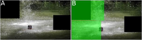
Fig. 9 Image belonging to the fountain class and its explanation after cover the significant and relevant areas marked in Fig. 8
As we know, the classification models do not always respond as we would like, and according to the previous example we can say that the use of the method proposed in this work, helps to explain the decision making of the model, as well as to the model improvement.
3.1 Impact of the Proposed Method
The relevance of the work presented here lies in the importance of knowing the reliability of the predictions given by a model, because, by definition, no model is perfect not even InceptionResnet, so when an incorrect prediction is made, it would be very helpful to know the reason and, thus, be able to improve the model.
If we ask a person to observe and identify the class to which the images in Fig. 10 belong, surely, they will answer to the cat’s class. However, the InceptionResnet model classifies these images at different classes: shopping_basket, quilt, and shoji, respectively.

Thanks to the visual explanation method proposed here, it is possible to know how exactly the model makes its classification decision as can be seen in Fig. 11. Then, the impact of the method is demonstrated.

Fig. 11 Visual explanations for the classes predicted by the InceptionResnet model for the images in de Fig. 10
Depending on the problem and the implementation of the model, this explanatory factor will be decisive in the improvement and appropriate uses of the model, in addition to contributing to its reliability.
3.2 Advantages of the Proposed Method
The proposed method solves one problem strongly present in other methods such as LIME [3] and RISE [4], that is the subjectivity of its results. Our method, with well-defined results according to the different proposed categories (significant, relevant, and futile), overcomes this problem as shown in Fig. 12.

Fig. 12 Explanations resulting from the application of different methods to the same image, which the Resnet50_places365 classifier model predicted as the main class patio, with a probability of 0.685. (A) Original image, (B) Explanation obtained by the proposed method, (C) explanation obtained by LIME, (D) Explanation obtained by RISE
For example, in the explanation obtained by LIME, it can be observed that regions that are not within the region marked in black are marked as important. It is also observed that this explanation is like the one obtained with our method, however, a difference in the results is that LIME does not mark well delimited regions that are considered important, that is, those regions in which a person could surely look at to determine that this image belongs to the patio class. It can also be perceived that the region resulting from the explanation with LIME is not well-delimited, since it shows a non-uniform region that includes certain confusing parts of the image which, as human beings, it is difficult for us to identify what they are, and consequently to obtain different conclusions for each observer who analyzes the results.
On the other hand, RISE generates an explanation very different from the explanations obtained with our method and with LIME. This could be somewhat confusing because in this explanation the regions of the greatest interest are highlighted as those marked in red and yellow, which as can be seen in Fig. 12 (D) are scattered throughout the image. Also, regions that could be of greater weight to reach a prediction are left out, for example, all the chairs and tables that are in the image, as well as part of the floor. Or, on the contrary, regions that might not be so important are considered, such as the window. Although, the window is part of the image, there is no clear relevance of it for the prediction, since a window can appear in different types of images that may belong to a different kind of patio. It is also noted that the effectiveness of RISE varies depending on the number of classes with which a model could classify an image, and that the time to generate an explanation turns out to be somewhat high compared to that of our method.
In contrast to the explanations obtained with LIME and RISE, it is observed that the proposed method delimits, with known and well-defined patterns (rectangles) that are also easy to perceive and understand for humans, those regions of interest that are important to classify this image as a patio. In these regions of interest, we can observe the chairs, the tables, the fireplace, the fence, the stairs, and even the floor, which has a typical finish that a patio could have. In addition, the importance of these regions is clearly differentiated and denoted by the color code (green, yellow, and red) defined according to their relevance (significant, relevant, and futile) for the prediction made by the model.
With this, there is a clearer intuition as to what the model has given more weight to perform its classification task. It can be seen, that unlike the proposed method, the explanations obtained with LIME and RISE are not so clear and are also subjective, i.e., the interpretation may be different depending on the observer. These methods also require a previous configuration of parameters, on which the obtained result depends.
3.3 Explanation by Class
Using the proposed method, it is possible to obtain not only the explanation of the class with greater probability but also of other classes with a slightly lower probability. For example, in the case of the InceptionResnet model that was trained to predict 1000 different classes, it may be the case that given an image, this image may belong in different degrees to different classes, and this belonging can be explained by applying our method. We show this in Fig. 13.

3.4 Method Validity
To verify the validity of the algorithm proposed in this work, a comparison process is carried out between the useful region obtained by the proposed algorithm, and the region selected by a person within that image. This region represents the most important region to determine whether an image belongs to one class or another. This comparison is carried out using the COCO data set, consisting of images tagged according to object within the image whose bounding box is marked by a human being, and it will be used as an indicator, since this region is what the network should ideally consider classifying the image.
In Fig. 14, four examples of images belonging to the COCO data set are shown, which have been marked and classified by a human being. These regions are compared against the explanation obtained by algorithm proposed here.

In Fig. 15, it is possible to observe that the useful region found by our explanation algorithm effectively surrounds the entire region marked by the human being. These results are that what would be expected from a good visual explanation algorithm, this of course, if the classifier model used is well trained. Otherwise, the utility of the explanation algorithm would change.

Keeping in mind the same logic, a subset of 200 different images of the COCO data set belonging to different classes were selected, and then a comparison with the proposed method explanation was made.
To carry out this comparison, the overlap of the two regions is measured as
The results obtained were favorable for all cases. We observed that the regions marked in COCO are always within the useful regions founded by the proposed explanation algorithm or
In addition to this and very importantly, the explanation is given in a non-subjective way using three clear, color-coded categories (significant, relevant, and futile), according to the relevance of the regions.
4 Conclusions and Future Work
In the present work, a new method is proposed to try to give a simple and easy to understand explanation about the predictions of an image classifier model. It has been demonstrated its validity, relevance, and usefulness. Furthermore, it has been shown clear advantages, such as solving the problem of subjectivity which is present in other explainability methods. This turns out to be very important since it is not subject to the interpretation of a certain person, so anyone will give the same interpretation to the explanation obtained and even it could be analyzed automatically, which has been left for future works. It was also shown that the performance of the proposed method is useful not only for correctly trained models, but also helps to understand the model prediction which sometimes goes against human intuition and thus be able to correct the model or data in a relevant way.
Table 1 shows a summary of the characteristics of the methods mentioned here (LIME, RISE) and the proposed method. The time column is based on the explanation obtained by each method for Fig. 12 (A) classified by the model as patio class, with a size of 640 x 426 px.
Table 1 Characteristics of methods
| Method | Year | Subjective |
Time (sec) |
Images | Text |
| LIME | 2016 | Yes | 105 | ✓ | ✓ |
| RISE | 2018 | Yes | 480 | ✓ | - |
| PROPOSED METHOD | 2021 | No | 25 | ✓ | - |
Future work will work towards improving the time and performance of the method, as well as its generalization to other types of classifiers.

