text new page (beta)
 English (pdf)
 Article in xml format
 Article references
 Send this article by e-mail
 Cited by SciELO
  Similars in
SciELO
Similars in
SciELO 
 Permalink
1 Introduction
Schizophrenia (SZ) is marked by a variety of behavioral deficits, including disturbances of attention, language processing, and problem-solving. SZ results in spontaneous brain activity without external interference [41]. It somehow overpowers the subtleness in the unity of consciousness and magnifies cognitive deficits [50]. At the same time, SZ is characterized by biological abnormalities, including disturbances in specific neurotransmitter systems (e.g., dopamine and norepinephrine) and anatomical structures (e.g., the prefrontal cortex and the hippocampus). The brain structure of SZ patients is different from a normal person. The lateral ventricles of SZ patients are enlarged compared to the normal patient.
Lateral ventricles generate cerebrospinal fluid that circulates different areas. When involved in speaking tasks, healthy control (HC) subjects have higher levels of salivary cortisol in comparison to SZ [25]. However, the behavior and biology of SZ have remained separate fields of inquiry. To bridge this gap between behavior and biology, irregularity in brain activity is often determined from EEG signals [58], and it helps to diagnose abnormality of brain activity in SZ patients who perceive the external activity as an internal activity. Evidence indicating crucial differences in the frontal lobes and temporal lobes. SZ patients show a different functioning of the frontal lobes and have a smaller temporal lobe structure in comparison to normal humans [46].
The delusional and hallucinatory experiences of SZ patients create critical reflection and prevent distinguishing the reality or validity of the experiences. Based on elusive, diffuse, defying description and understanding, the psychotic experiences arise [44, 37]. SZ may be positive or negative according to the patient’s psychotic experiences. Positive symptoms of SZ implies talking nonsense words, changing thoughts, moving slowly, unable to take decisions, forgetting, having problems in the sense of feelings, hearing, and looking, etc. Negative symptoms of SZ imply a deficiency of emotions, energy, speaking, motivation, interest in life, withdrawal from family, friends, and social activities, etc. [25].
The human brain’s electrical activities can be measured through Electroencephalography (EEG), which is useful in detecting SZ. The international system “10-20” describes the location of scalp electrodes for an EEG test. Identification of SZ patients can be found out by analyzing the complexity of the EEG signals [58]. They worked on EEG signal complexity to find out SZ against normal subjects. They found out that it is possible to detect SZ with an analysis of EEG signals complexity at the time of mental activity.
For monitoring and diagnosing pathological/psychological brain states, EEG is a practical tool, and non-linear-based algorithms can interpret these EEG signals to detect SZ. For SZ diagnosis, combine features of signals shows 100% accuracy and concluded that it is possible to detect it with non-linear combinations of features instead of linear [22]. The SZ can be detected by analyzing EEG signals with 100% accuracy, and the potential of 16 electrodes can be analyzed for reducing the computational complexity [53].
When analyzing EEG signals, the value of Shannon entropy of HC is more significant in comparison to SZ which implies, the higher information possible to get from HC to SZ patients [39]. The EEG data from 877 SZ and 753 normal control SZ subjects (NCSs) shows there are linear and nonlinear abnormalities in SZ, and these abnormalities help to detect SZ in the pathophysiology test [33]. The study of brain activity of two groups, an SZ group, and an HC group, shows that visualization of complexities of EEG signals of 16 channels helps to classify SZ patients and HC subjects [31].
EEG data (256 channel records) of 38 SZ patients and 20 HC are classified using supervised machine learning techniques with accuracy in classification [59]. An experiment with 40 SZ patients and 12 HC participants showed that EEG features consistent with low-frequency activity for memory encoding, memory retention, and elevated resting in the case of SZ [24]. A further study of 45 SZ and 39 HC subjects, has shown that 16 channels of EEG signal complexity help psychiatrists diagnose patients with SZ [32]. With 15 SZ and 18 HC subjects, three EEG analysis methods, complexity, variability, and spectral measures are studied and distinguished the features for SZ [48]. It was an experiment with 12 channel signals from 4 SZ and HC subjects, which has shown frontal lobe channels have increased in delta and theta waves the occipital lobe have decreased in alpha waves in case of SZ in comparison to HC patients [2]. 19-channel EEG signals were collected from HC and SZ with different kernel-based classifiers experimented with an accuracy of classifications [23].
To automatically detect SZ from the EEG signals data, we can use different machine learning tech-niques [49]. One of the advanced machine learning techniques, SNN shows excellent performance on detecting and classifying the EEG signals [42, 20, 5, 51, 35, 21, 28, 17, 16, 56, 27, 7, 47, 29, 38]. SNN with deep learning in the hidden layer has an efficiency to classify and predict the target in supervising form [57, 61]. The SNN model can be formulated with a different concept of probability of different neural models and can classify according to requirement [42, 20].
We have found a variety of different machine learning classifiers are implemented with EEG signals to identify the SZ patient’s EEG recording distinguish structure [59, 24, 48, 23, 43, 45, 14, 9, 10, 52, 62, 6, 1, 34, 36], but particular abnormalities in the signals are not taken into consideration. SNN technique can emphasize the spectrum pattern to study the abnormal spikes generated in the case of SZ in comparison to the HC subject. Hence the encoding of the particular abnormalities in terms of spikes of the different channel which are an abnormal indication of signals for SZ and doing manipulations with the spikes, it can give better result in less manipulation. And the spikes’degree of importance in the classifier is included with the training of LSTM, which sequentially considers the neurons’spikes since SNN has the advantage of spiking identification and is trained with the deep learning approach.
EEG signals collected from scalps show brain activities, and by analyzing that spectrum sharply, we can visualize the abnormal activities and slow processing of neurons.
The SNN approach first emphasis going through the deep dataset pattern to generate spikes and EEG recording signals oscillations are fluctuated according to the brain electrical activities in a time series, so it is a suitable approach to model an SNN for identifying SZ electrical activities in the brain from EEG signals and predict the SZ patient and HC.
[15] included 34 SZ and 33 HC evaluated somatosensory potentials evoked through the right median nerve that have a deficiency in information processing for SZ patients. [55] included 32 SZ, 28 first-degree relatives, and 31 HC participants with 128 channels recording it was found that lower power spectral density in the case of SZ.[60] summarised that TMS and EEG could help for pathophysiological information processing to find out deficits in SZ patients. With the identification of SZ patients through EEG recording, it is possible to give treatment with neurofeedback (NBF) and can have a successful performance [54]. The EEG signals of 256-channel found out the abnormalities and slow-wave oscillations for SZ in comparison to HC [11].
EEG signals 9 deficit SZ, 10 non-deficit SZ and 10 HC showed alpha band time-series signals difference in the frontal lobe [12]. EEG recording is simple, low-cost, shows hallucinations and abnormalities for SZ, and through it, possible to analyze the posterior temporal lobes connectivity and functional associations of auditory processing [18]. The signals from the cerebral cortex show the symptom of functional impairment association for SZ patients, and a review highlighted the way of impairment in cortical network imbalances and abnormalities in signals and disturbances functional output [30]. A study of 64 EEG channels recording showed low frequency, abnormal slow frequency of beta, and unique endophenotypes for SZ subject [40].
2 Methods
Our objective is from EEG recording of SZ patients in a time interval are analyzed to manipulate the spikes where spike implies the units of frequency and prediction is generated whether the spikes from different neurons in the time intervals are combinedly showed the symptom of spontaneous schizophrenia patients (SZ) or control healthy subject (HC). The prediction accuracy and evaluation are manipulated to check the performance. We have used SNN with Temporal contrast, pSNM, SpikeProp, and LSTM to classify HC and SZ.
For the implementation, we have used Python 3.6, Excel, and CSV files with Windows 10 OS.
We have taken the time series data set of EEG recordings from the Kaggle database1. A simple button-pressing task is organized to collect EEG data from 32 HC subjects and 49 SZ patients in which subjects either pressed a button to immediately generated a tone, heard the tone, or pressed a button without tone generation and the corollary discharge is studied in people with SZ comparison to HC. Between 1 to 2 seconds, the subjects pressed a button with the sound of 1000Hz, 80dB, and there was no delay between button press and tone generated.
The task was of 100 tones deliberations. The EEG data are collected from 64 channels, but after pre-processed, we have only nine electrodes to be considered.
The pre-processing is applied with raw EEG data of each subject. The sequence of pre-processing followed is a high-pass filter of 0.1Hz, the outlier channels of continuous EEG data are interpolated, data recorded in 3 seconds (1.5 seconds before an event and 1.5 seconds after an event)and a total of 9 seconds per subject, the baseline of signals corrected -100ms to 0ms, muscle, and high-frequency white noise artifacts are removed using canonical correlation analysis, outliers single trials are rejected, a spatial independent components’analysis is used to remove some components, and within single trials, outlier channels are interpolated.
Event-Related Potentials (ERPs) are calculated by averaging across trials for every sample in the time series, separately for each subject, electrode, and condition. Hence the ERP data is a derived data that includes 9 electrodes Fz (Midline Frontal), FCz (Midline Frontal Central), Cz (Midline Central), FC3 (Frontal Central 3), FC4 (Frontal Central 4), C3 (Central 3), C4 (Central 4), CP3 (Central Parietal 3), CP4 (Central Parietal 4). Since SZ patients show a different functioning of the frontal lobes and have a smaller temporal lobe structure in comparison to normal human [14], so the above 9 channels included for the experiment is justified for classifying SZ and HC. The nodes are pointed in Fig. 1. When the button-pressing task is performed by the 81 subjects, their EEG recording is represented in Fig. 2, and the recordings of channels are depicted with HC subjects against SZ patients in Fig. 3.

Fig. 1 The image is a brain structure of the SZ patients in comparison to non -schizophrenia. The upper image is the structure of the brain. The lower image is pointing to the locations of nodes from where the nine EEG signals are collected for the experiment. Since the abnormal structure of frontal and temporal lobes of the brain causes SZ abnormalities, so signals of electrodes Fz (Midline Frontal), FCz (Midline Frontal Central), Cz (Midline Central), FC3 (Frontal Central 3), FC4 (Frontal Central 4), C3 (Central 3), C4 (Central 4), CP3 (Central Parietal 3), CP4 (Central Parietal 4) are analyzed. Regions of interest are placed with the electrodes where the Left frontal is indicated with blue color, the Frontal is indicated with red color, the Right frontal is indicated with purple color, and the Central is indicated with yellow color
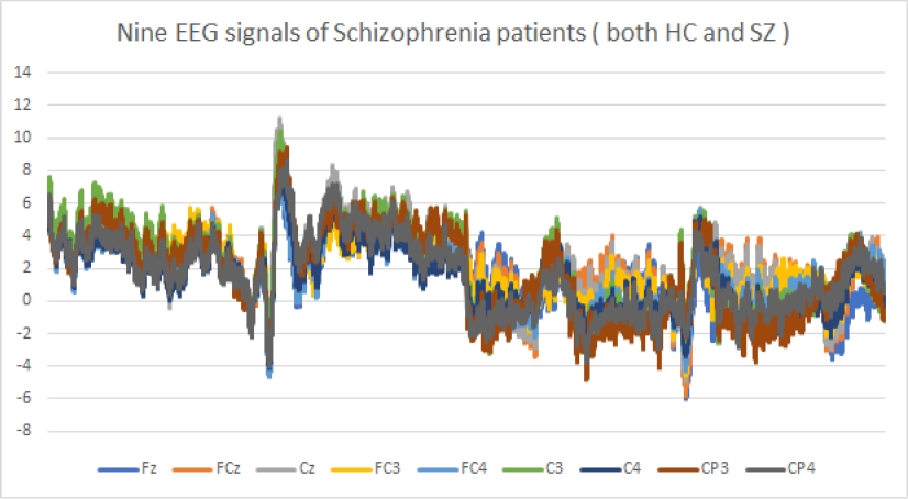
Fig. 2 EEG signals pattern of subjects, which is either SZ or HC. The image shows nine channels Fz electrode, FCz Electrode, Cz Electrode, FC3 Electrode, FC4 Electrode, C3 Electrode, C4 Electrode, CP3 Electrode, CP4 Electrode signals. Maximum channels have signals’ frequency of approximately 7Hz
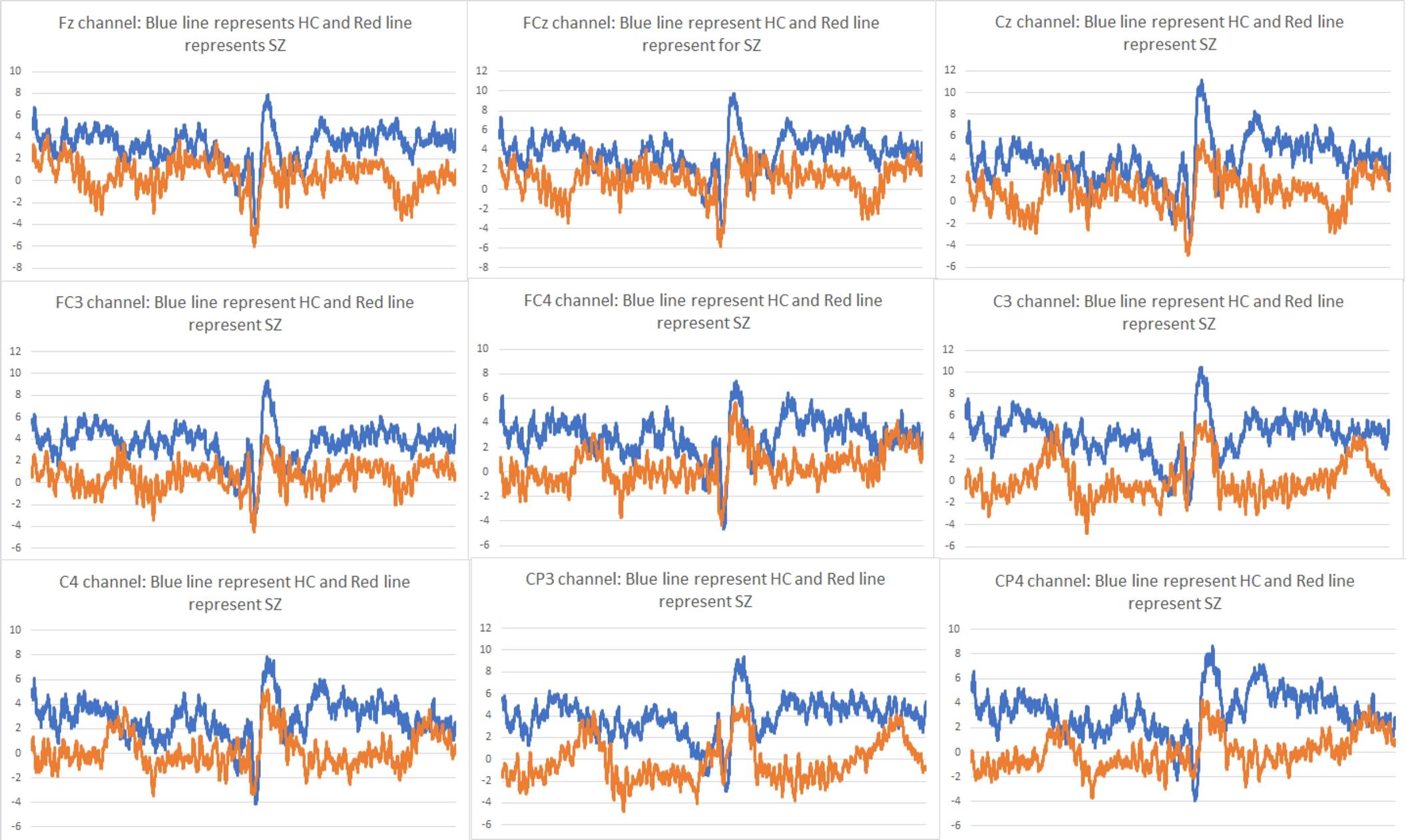
Fig. 3 The graph represents the signals of channels Fz electrode, FCz Electrode, Cz Electrode, FC3 Electrode, FC4 Electrode, C3 Electrode, C4 Electrode, CP3 Electrode, CP4 Electrode according to HC and SZ patients. Approximately all frequency of channels is about 7Hz, where HC patients have approximately more than 2Hz, and SZ patients have approximately less than 2Hz
Fig. 4 shows the nine EEG signals of HC subjects, and Fig. 5 shows the nine EEG signals of SZ subjects and Fig. 2 shows the nine EEG signals of subjects that are of both HC and SZ subjects.

Fig. 4 The graph of nine EEG signals of channels Fz electrode, FCz Electrode, Cz Electrode, FC3 Electrode, FC4 Electrode, C3 Electrode, C4 Electrode, CP3 Electrode, CP4 Electrode for HC subjects
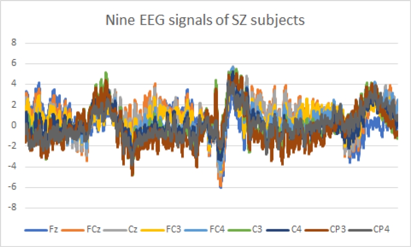
Fig. 5 The graph of nine EEG signals of channels Fz electrode, FCz Electrode, Cz Electrode, FC3 Electrode, FC4 Electrode, C3 Electrode, C4 Electrode, CP3 Electrode, CP4 Electrode for SZ subjects
All description mentioned above is extracted from the data set, and the data description is summarized in Table 1.
Table 1 The information of 81 subjects EGG recording data from nine channels (Fz, FCz, Cz, FC3, FC4, C3, C4, CP3, CP4) are summarised. Also, the subject’s information is noted
| Information about subjects and their EEG recording | |
| Number of subjects | 81 |
| Number of males | 67 |
| Number of females | 14 |
| Maximum age of subjects | 63 |
| Minimum age of subjects | 19 |
| Number of control subjects | 32 |
| Number of uncontrol patients | 49 |
| Number of electrodes recorded | 64 |
| Number of electrodes after filtered | 9 (‘Fz’, ‘FCz’, ‘Cz’, ‘FC3’, ‘FC4’, ‘C3’, ‘C4’, ‘CP3’, ‘CP4’) channels. |
| Time interval recorded per subject | 9000ms approximately |
| Different conditions | control, uncontrol |
| Frequency of Channels recorded | Each 1.5ms approximately |
| Each subject has instances | 9,000 approximately |
| Total number of instances | 7,46,496 |
3 Results
EEG data are recorded in time intervals of 13,500ms for approximately every subject. It is a study that approximately all SZ patients have 7Hz or less than 7Hz frequency. In contrast, maximum HC subjects have higher than 2Hz, and maximum SZ subjects have less than 2Hz for each of the nine channels (from the fitted curve in Fig. 3). Using the encoded Temporal contrast method with a threshold value of 2Hz, spikes are generated from the recorded signals of nine channels. The spikes rates for HC plotted in Fig. 6, and SZ subjects are plotted in Fig. 7. Finally, we have derived the average spike rate for HC and SZ patients for every nine channels, which are depicted in Fig. 8.
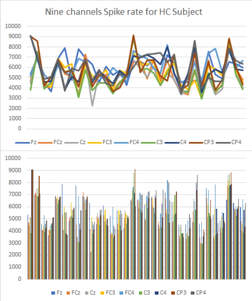
Fig. 6 The graph and bar representation of spike rates according to channels Fz electrode, FCz Electrode, Cz Electrode, FC3 Electrode, FC4 Electrode, C3 Electrode, C4 Electrode, CP3 Electrode, CP4 Electrode for HC are plotted

Fig. 7 The graph and bar representation of spike rates according to channels Fz electrode, FCz Electrode, Cz Electrode, FC3 Electrode, FC4 Electrode, C3 Electrode, C4 Electrode, CP3 Electrode, CP4 Electrode for SZ are plotted
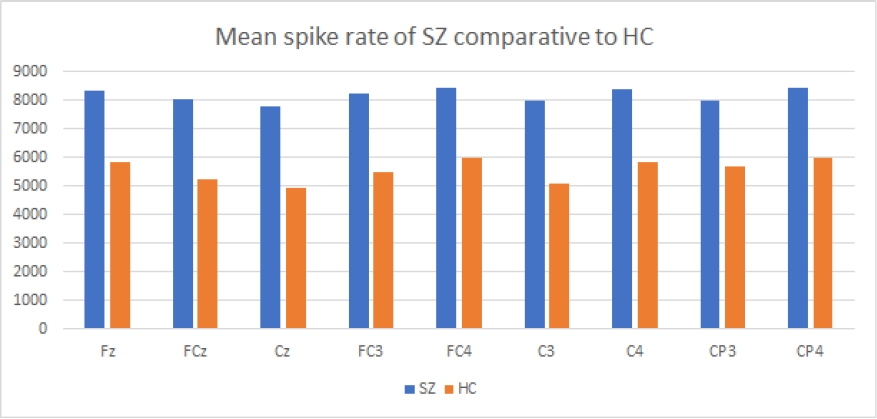
Fig. 8 The bar diagram represents the mean spike rate of channels Fz electrode, FCz Electrode, Cz Electrode, FC3 Electrode, FC4 Electrode, C3 Electrode, C4 Electrode, CP3 Electrode, CP4 Electrode according to both HC and SZ. It is found that the average spike rate of SZ is more comparable to HC for every channel
The probability of spikes towards SZ patients is calculated for each channel using Poisson distribution probability as defined in equation 4, and we have got the probability of SZ patients according to each channel independently. Probabilities to be an SZ patient on behave of each channel are represented in Fig. 9 for 81 subjects where 32 are HC subjects, and 49 are SZ subjects. After calculating probability, we have combined the nine-channel probabilities re-currently or sequentially using supervised machine learning techniques LSTM.

Fig. 9 The diagram represents the spike probability of channels Fz electrode, FCz Electrode, Cz Electrode, FC3 Electrode, FC4 Electrode, C3 Electrode, C4 Electrode, CP3 Electrode, CP4 Electrode independently where spikes indicate the patient is SZ
The LSTM is used two times, with 110 epochs to optimizes the weights and classifying. We have taken 50% of the data set for training and 50% taken for testing. Using the 1-fold cross-validation method, 96% accuracy is predicted when trained with LSTM to predict an SZ patient. Also, the ROC AUC curve shows a 100% true positive rate, which is depicted in Fig. 10. After trained with the LSTM model, every 81 subjects are evaluated with sequential combinations of nine channels, and the result is depicted in Fig. 11.
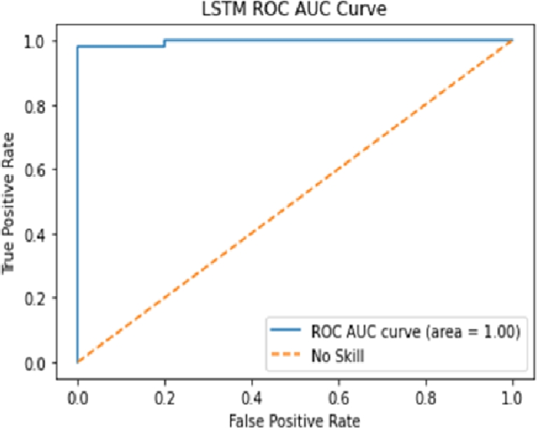
Fig. 10 The output of the LSTM implementation result is depicted in a ROC-AUC curve. The blue line shows the performance of the classifier, and the red line indicates the worst performance borderline. The ROC-AUC curve area shows 1.00. Hence 100% true positive rate and the classifier performance is excellent
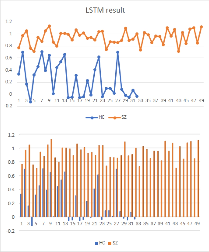
Fig. 11 After implementing LSTM on nine channels (the probability of spike independently for each channel) which combinedly predict a result as the chances of the spike to be an SZ patient, the probability is depicted on the above figure in terms of the graph as well as a bar for 32 HC and 49 SZ patients
Finally, decoding the temporal contrast method generates the output spikes with the threshold for finding the spikes is 0.707. Spikes predict SZ patients. Thus, this SNN model shows 100% accuracy with a threshold value of 0.707 when validated with 81 subjects with a one-fold cross-validation method and taking 50% as a training subset and 50% as a validation subset. The result is showing that the classifier and predictor are with 100% accuracy, and the performance shows the robotic result, as shown in the following confusion matrix and Table 2. Confusion Matrix:
4 Discussion
The Kaggle database of EEG recording of SZ disorder patients was implemented with traditional classifiers SVM, RF, ANN, and NB by [4]. We have proposed a probability SNN model for the classification of EEG signals collected from the subjects suffering from spontaneous and controlled SZ.
Different works are found relating to SZ disease, EEG signals, machine learning classifiers, recurrent neural network LSTM, and SNN. A study of nine nodes Fz, FCz, Cz, FC3, FC4, C3, C4, CP3, CP4 are channels extracted from patients having an abnormal brain disorder. The graphical representation Fig. 2 shows that the data used are data extracted from patients who have an abnormal brain disorder since the readings of each of the 9 electrodes are below 7Hz. Usually, the frequency of the waves of an awakening adult is 8Hz and above, and wave frequency of 7Hz or less is shown with abnormal in awake adults or children or asleep adults who are asleep [26]. EEG recording of 23 channels of 78 SZ patients is analyzed, and in conclusion, that from EEG recording, it is possible to identify SZ patients [58].
We have taken the EEG dataset of the SZ people with control and spontaneous attitudes for our experiment. Different machine learning techniques classify and predict SZ patients. The study of EEG signals of 31 SZ patients is analyzed to classify as controlled and spontaneous patients. 22 channel recording features are considered with the classifiers BDLDA, standard LDA, Ada Boost, SVM, FSVM, and BDLDA shows robustness performance [8]. Some papers concern the diagnosis of SZ patients suffers from several cardinal problems, and a classifier called TFFO proposed with three number of well-located electrodes [19].
The said 3rd generation machine learner pSNM, a model type of SNN, may be implemented for classifying EEG recordings. LSTM RNN model is proposed for EEG data classification.
Low/high arousal, valence, and liking are the feature of emotion and, according to EEG recordings, are different, which are classified using LSTM and given good accuracy compared to other machine learning methods [3].
100% accuracy with specificity, sensitivity can be found out using RNN on EEG signals of epileptic seizer detection [38]. Hence, after deriving spikes from EEG signals, it is possible to use LSTM RNN for classification.
The SZ patient’s EEG data set collected from the Kaggle database is of 81 subjects with 49 SZ and 32 HC patients. Spikes are generated from each channel using an encoded temporal contrast method.
The mean spike rate is manipulated to evaluate the probability, and LSTM is implemented for sequentially combining each channel probability to evaluate and predict the SZ patient.
LSTM trained the classifier with 97% accuracy after 110 epochs with a 100% true positive rate. Then the decoded temporal contrast method is used to predict the result or state of the SZ subject. Finally, 100% accuracy is showed with the pSNM model of the SNN. Since the pattern of EEG signal depends on brain electrical activity, so generating spikes using different rate codes with the mathematical formulation is a challenging task. By emphasizing those formulations, in the future, we may model a classifier having robust performance.
Although SNN discussed in the Appendix is not implemented with EEG signals of SZ patients, we have found out some experiments on EEG signals of SZ patients with Deep learning, NN, and other classifiers.
The same dataset was also implemented with CONVNETS deep learning approach and showed 63% accuracy in classifying after 100 epochs2. Implementation of Kernel-SVM with 58 subjects’ EEG recordings, the experiment has concluded with the classification of SZ against healthy subjects is possible with machine learning (ML) techniques [59].
ML technique SVM has experimented with 52 subjects, and the EEG recordings of them are classified according to SZ and HC subjects with 74% accuracy [24]. EEG signals of 33 subjects are classified with ML technique K-NN and with 94% accuracy, it has classified SZ and HC subjects [48].
The traditional machine learning techniques were implemented with 19 EEG recording channels to classify SZ and HC patients and have shown with a certain level of accuracy to classify successfully [23].
A convolution neural network model is trained with EEG data of SZ and has scored better performance and is suggested to identify SZ with the pathological study of scalp areas and SZ conditions [36].
ANN classification technologies can ably classify symptoms of brain disorder in relating to SZ, and it also summarized that more computation is required in ANN for classification [34]. A study was carried on children’s EEG recording to find out the development of SZ on them, and recurrent convolution neural network and traditional machine learning are implemented with it. The conclusion suggests that the capability of deep learning models with EEG recording allows detecting the psychosis of children at the early stages [1]. An experiment on 28 participant’s EEG spectrum with ML random forest classifier showed 96% accuracy on classifying 14 SZ and 14 HC subjects [9].
CNN is trained with two EEG datasets and successfully classified SZ and HC subjects with a level of accuracy 95% and 97% and reach after the relationship between frequency of signals and SZ and showed from images of frequency, the difference between SZ and HC subjects [6]. CNNV-RF and CNNV-mSVM are implemented with resting-state EEG streams and found out well performance in classifying schizophrenia patients [14].
A deep learning model MDC-CNN is imple-mented with EEG recording to classify SZ and HC subjects and has 91% accuracy[45]. An eleven-layered convolutional neural network (CNN) model was experimented with 14 SZ and 14 HC subjects and has shown an excellent performance of above 85% accuracy in classifying [43]. The 19 channels EEG signals from 14 healthy and paranoid schizophrenia subjects are classified with random forest machine learning techniques with 100% accuracy [10]. An approach DNN-DBN is experimented with for classifying SZ and HC subjects, and well performance was shown in comparison to traditional machine learning [45].
A convolutional neural network approach was implemented to classify SZ and HC subjects, and this ANN has shown successfully in classifying with above 86% accuracy [52].
Random forest classifier has implemented with 9 EEG recordings from 81 subjects and was classified successfully [62].
5 Appendix
5.1 Spiking Neural Network Algorithm
The machine learning technique SNN has three layers, i.e., the input layer, an output layer, and the hidden layer. The input layer containing input data, which generates the spikes, the hidden layer train the spikes, and the output layer also generate the spikes of target evaluations.
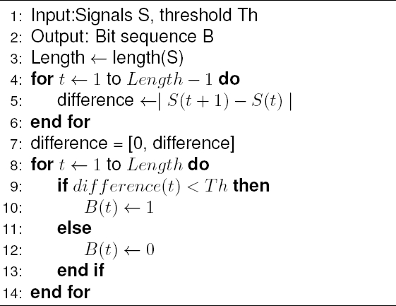
The encoding procedure transfers the real value of input information to discrete sequences of spikes as a new format of inputs to SNN models. The Temporal contrast or Threshold-based encoding method is a simple method to generate the spikes.
The encoding of spikes is generated using equation 1:
where S(ti) units value at time interval [t(i−1), ti] and θ is the threshold value.The output decoding procedure transfers the real value of output information to a discrete sequence of spikes. The decoding of the spike is found out following equation 2:
where P (ti) chances of the spike at time ti and θ is threshold value. The probabilistic spiking neuron model (pSNM) has considered the following steps to model a spiking neural network:
Probability
The post-synaptic potential (PSP) reaches the threshold (Pi(t)) where PSP is found out by sum total of the probability of the post-synaptic neuron ni .
Thus, the graphical representation with nine neurons with pSNM is elaborated in Fig. 12.

Fig. 12 N1, N2, N3, · · · , N9 are the inputs from which spikes generated, then it’s probability are manipulated using poisson distribution as P (m1), P (m2), · · · , P (m9) combine all probabilities using advance RNN, LSTM to find the probability of spike and finally threshold value Pi(t) decides whether it‘s the spike of disease. Evaluate P SPi(t) using LSTM
The state of postsynaptic neurons is representing the probabilities of the spike on behave of the nine neurons. The postsynaptic potential P SPi(t) is calculated using equation 3:
The proposed model is finally manipulated for decoding with threshold value evaluation on the basis of equation 3, where ej = 1 if spiking is emitted and 0 otherwise.
where λ is the mean value of the existing population of spikes.
Learning in this SNN model follows SpikeProp where SpikeProp refers to the number of firing detection for a given set of input patterns. From the input values, we get post-synaptic values that generate the fires. The functions of error minimization and weight values that connect pre and post-synaptic are used to interpret the firing spikes. Recurrent Neural Network (RNN) can solve the purpose of sequence handling to learn the model. RNN is the sequence of the same network with each network passing information to the successive network. A modified version of RNN, LSTM is selectively considered the previous values of the features. LSTM is comprised of different cells mechanism shown in Fig. 13.
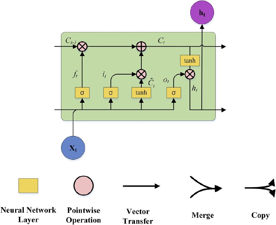
Fig. 13 Each neuron evaluation of recurrent neural network model LSTM where neuron evaluation depends on previous neuron evaluation value, evaluation of current neuron value and importance value of neuron. Input gate is for previous neuron evaluation, output gate is for evaluation of current neuron, and forget gate is for importance value for neuron [35]
The neuron blocks are manipulated with three major mechanisms as forget gate, input gate, and output gate as shown in Fig. 14. Two well-known functions the hyperbolic function tanh and sigmoid function are used in a cell of neural network. For a cell, three gates are used which are manipulated according to equations 5 to 9. Equation 5 represents the forget gate which generates the value between 0 and 1 for the state value of the cell. Here 1 is interpreted as the state value is completely kept and 0 says the state value is completely not considered and the middle value between shows the degree that cell state value is considered.

Then the input gate is to be considered using the equations 6 to 8. Here the sigmoid function is used to determine which value should be kept, as define equation 6 and tanh function creates a vector of state values as equation 7 to consider state value. Finally, the state value of the cell evaluated considering both equations 6 and 7 as presented in equation 8.
Next output gate is evaluated using the equations 9 and 10 where ot is updated out value and ht is the updated state value for the cell:
where h(t−1) is the state value of the previous neural cell, xt is the input value for the existing cell, bf ,bi ,bc, and bo are biased values, wf, wi, wc and wo are the weight values, σ is the sigmoid function where σ(v) = 1/(1 + e(−v), tanh is hyperbolic function where tanh(v) = (e2v − 1)/(e2v + 1).
5.2 Gradient Descent Optimization Method
We have a cost function define as equation 11:
where Y′ are the predicted values for the classification model and Y is the actual values that are observed. N is the total number of training data and error is
5.3 Evaluation Method
The machine learning skills can be evaluated using the cross-validation method which is a statistical procedure. According to the procedure of the cross-validation method, the data set is divided into two sets i.e., the training set and testing set. The classifier is trained with a training subset of a dataset and the classifier skills are evaluated using the testing subset of the data set. This method is said as a one-fold cross-validation method. This procedure can be followed more than one time to evaluate the classifier more accurately.
If we follow the method k times then it is called the k-fold cross-validation method. In the k-fold cross-validation method, we divide the dataset into k parts where k-1 parts are taken for training the classifier and one part is taken for evaluating the classifier. This procedure is followed k-1 times with each time one different subset is taken for validating and k-1 subset are taken for training. Finally, the average of testing values is considered as the skill of the classifier.
The receiver operating characteristic curve (ROC) is depicted for measuring the performance of a classification machine learning method with a dataset at all various thresholds generated for the classifier. It is plotted by manipulating the true positive rate (TPR) and false positive rate (FPR) where FPR is plotted on the x-axis and TPR is plotted on the y-axis. We can measure the TPR and FPR using equations (12, 13):
where TP stands for observed true positive, TN stands for observed true negative, FN stands for observed false negative, and FP stands for observed false positive. The area under the ROC curve (AUC) represents the quality of the classification model by ranking random positive data against random negative data. The value of AUC-ROC lies between 0 and 1. If the value is 1.0, the prediction is 100% true, if the value is 0.0, the prediction is 100% false and if the value lies between them, then the prediction truthiness is accordingly interpreted.
The summary of our work is presented in Fig. 15.
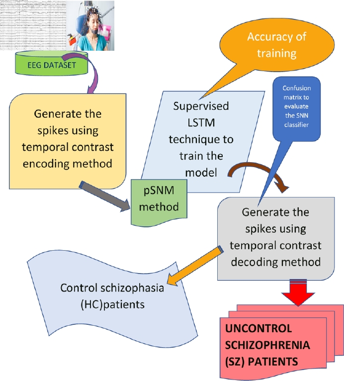
Fig. 15 We have collected the EEG recordings which are already pre-processed. According to the research experiments’ opinion, we have analyzed the data and used the temporal contrast method to generate spikes. Then each channel spikes are combinedly interpreted using LSTM recurrent method. Again, the contrast method has been used to generate the predicted spikes which show uncontrolled schizophrenia
The prediction results on a classification model are summarized in a confusion matrix as in Table 3.
Table 3 Representing the evaluation matrix of a classifier trained using the machine learning method
| Positive rate prediction | Negative rate prediction | |
| Real positive rate | TP | FN |
| Real negative rate | FP | TN |
It shows the ways the model is confused in prediction and also make ready to face errors and type of errors that are being made.
Then we can calculate accuracy, recall, precision and F-measure as follows:
If the classifier shows 99% accuracy it is interpreted as excellently trained with the machine learning technique. The class prediction correctly recognizes if we have a high recall value. High precision indicates positive label prediction is positive and there is a small number of false positives. The high F-Measure shows nearer to the higher value of Precision or Recall.
5.4 Algorithmic Representation of the Proposed Approach
Our proposed approach is based on SNN, where each neuron or channel is interpreted recurrently one by one using LSTM. For the simulations, we have followed the steps as defined below:
— Step 1. We have generated the spikes from each signal in a specific time interval using a temporal contrast method where the temporal contrast encoding algorithm is as in Algorithm 1.
— Step 2. For time intervals, we find out the rate code by calculating the average number of spikes generated for a time interval.
— Step 3. Using Poisson probability distribution, the probability of spike is calculated for each neuron.
— Step 4. Using recurrent algorithm LSTM, all probabilities generated from each neuron are combined to predict the probability of spike to be simulated for indicating the abnormality of the signal.
— Step 5. Again, temporal contrast decoding algorithms are implemented to conclude whether an abnormality signal is the prediction of an event where the event may be a symptom of SZ. The temporal contrast decoding algorithm is as Algorithm 2.
— Step 6. Spike in term of 1 concluded the disorder symptoms (SZ), whereas 0 indicates the normal control symptom (HC).