On the Paraconsistent Logic CG'3

Pérez-Gaspar, Miguel; Borja Macias, Veronica; Bárcenas, Everardo; Pérez-Gaspar, Miguel; Borja Macias, Veronica; Bárcenas, Everardo

doi:10.13053/cys-25-2-3363

Services on Demand

Journal

Article

Indicators

Cited by SciELO
Access statistics

Computación y Sistemas

On-line version ISSN 2007-9737Print version ISSN 1405-5546

Comp. y Sist. vol.25 n.2 Ciudad de México Apr./Jun. 2021 Epub Oct 11, 2021

https://doi.org/10.13053/cys-25-2-3363

Report on PhD thesis

On the Paraconsistent Logic CG'₃

Miguel Pérez-Gaspar¹

Veronica Borja Macias²

Everardo Bárcenas¹^*

^¹ Universidad Nacional Autónoma de México, México. miguel.perez@fi-b.unam.mx, ebarcenas@unam.mx

^² Universidad Tecnológica de la Mixteca, México. vero0304@mixteco.utm.mx

Abstract

Paraconsistent logical systems are well-known reasoning frameworks aimed to infer new facts or properties under contradictory assumptions. Applications of these systems are well known in a wide range of computer science domains. In this article, we study the paraconsistent logic CG'₃, which can be viewed as an extension of the logic G'₃. CG'₃ is also 3-valued, but with two designated values. Main results can be summarized as follows: a Hilbert-type axiomatization, based on Kalmar's approach; and a new notion of validity, based on also novel Kripke semantics.

Keywords: Many-valued logic; paraconsistent logic; Kripke-type semantics; Hilbert calculi; CG'₃

1 Introduction

Many valued logics, as classical ones, are based on the principle of truth-functionality.^¹ In the classical approach, there are only two truth values, falsum and verum, which are commonly written "0" and "1". Contrastingly, in many-valued logics more than two truth values are considered. A survey on many-valued logics may be found in ^[⁹^]. Originally motivated by philosophical aims, many-valued logics are also inspired by formal technical concerns regarding functional completeness.

Among the first applications of many-valued logics, one may found hardware design. Analogously, as classical logic is used as a technical tool for the analysis and synthesis of electrical circuits built up from switches with two stable states, denoting voltage levels, many-valued logic can be used as general model of electrical circuits with more than two stable states. This application field of many-valued logic is called many-valued switching ^[⁶^].

We now list some current state-of-the-art applications of many-valued logics in artificial intelligence: imprecise notions inherently tied to commonsense reasoning in expert systems, can be naturally modeled via fuzzy logic. Inference systems for many-valued logics, fuzzy logic in this context, can then be used as reasoning frameworks in expert systems ^[⁹^]. A relatively recent research perspective in the AI setting, concerns the many-valued generalization of description logics, well-known as the reasoning foundation of the semantic web ^[¹⁰^].

In ^[¹⁴^], it is extensively reported on non-monotonic reasoning based on paraconsistent logics. In particular, it is proposed a logic programming semantics based on the paraconsistent logic G’₃. This is called G’₃-stable semantics. Inconsistent and vague domains can be naturally modeled with this G’₃-stable semantics.

In ^[¹⁶^], Priest affirms that one of the motives of da Costa, to build the paraconsistent logic C_w, was dualizing the negation of intuitionistic logic. Intuitionistic logic is a logic that allows for "truth-value gaps"; for example, the Law Excluded Middle fails. The logic C_w achieves this but with explicit costs; for example, the substitution of provable equivalents fails. Da Costa proceeded axiomatically, preserving the positive part of intuitionistic logic, and changing the axioms of negation.

But the various semantics for intuitionistic logic suggest other ways of pursuing da Costa's goal. Evidence of this is the paraconsistent logic created by Priest that arises when dualizing the modeling conditions for the negation in Kripke semantics for intuitionistic logic. This new system is called da Costa logic daC. We can find at the end of ^[⁷^{] section 2} a brief study of extensions of fragments of Heyting Brouwer Logic. This is the case of the family of logics daCG_n; each an extension of daC characterized by a Kripke frame for daC, which is linearly ordered and has n - 1 points. We have that G’₃ corresponds to daCG₃, and clearly, the characterization agrees.

In ^[¹⁵^], Osorio et al. define G’₃ through its multi-valued semantics. CG'₃ is an extension of G'₃^[¹³^]. In contrast with G'₃, whose designated value is 1, CG'₃ has 1 and 2 as designated values. It is important to note that G'₃ is not comparable with Godel logic G₃. In Figure 1, we present some logics related to CG'₃ where the arrows mean contention.

Fig. 1 Comparison of G'₃ and CG'₃ with other logics

The structure of the document is as follows. In Section 2, we present the definition of CG’₃ from many-valued semantics. In Section 3, we give the formal axiomatic theory L for CG’₃ and examine some interesting properties of L, and we close the section seeing that L is sound and complete concerning CG’₃. To prove that L is complete, the authors follow the procedure of completeness proof used for classical logic given in ^[¹²^] and originally due to Kalmar. This method has been used in other many-valued logics, see ^[¹^,¹¹^]. In Section 4, we show the semantical similarities between CG’₃ and the many-valued logic Ł3. In Section 5, we introduce the Kripke-type semantics to CG’₃, in two different ways.

2 Many-Valued Semantics for CG’₃

We first introduce the syntax of the logical formulas considered in this paper. We follow standard notation and basic definitions as M. Osorio in ^[¹⁵^].

The following symbols will be used for logical connectives: ˄ (conjunction, binary); ˅ (disjunction, binary); ↔ (biconditional, binary); ¬ (weak negation, unary); ∇ (inconsistency operator, unary); ~ (strong negation, unary) and ⊥ (bottom formula, 0-arity).

Fix the propositional language L whose primitive symbols are:

— the variables p₀,p₁,…;
— the connectives: ˄, ˅, ¬ , and → ;
— the punctuation marks: ( and ),
— the formulas of L are defined inductively:
- — all the variables in L are atomic formulas o simply atoms;
- — if φ and ψ are formulas then φ∧ψ, φ∨ψ, and φ→ψ are also formulas.

One of the most popular semantics for many-valued logical systems is the standard logical matrices. The most appropriate way to define semantics for a logic of many-values is through a logical matrix characteristic from its language, that is:

— the set of values of truth (domain),
— the set of designated values, which form a subset of the set of truth degrees and act as substitutes for the traditional truth value verum,
— the functions of degree of truth interpreted by the propositional connectives.

A well-formed formula φ of a propositional language counts as valid under some valuation v^² if and only if it has a designated truth value under v. And φ is a tautology if and only if it is valid under all valuations, and we denote this by ⊨φ.

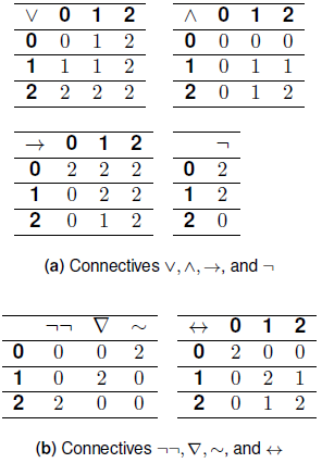
The paraconsistent logic CG’₃ is introduced in ^[¹³^] and is given, by the matrix M=D,D*,F; where D = {0,1,2} is the domain, D* = {1,2} is the set of designated values, and F is the set of truth functions for the connectives {˄, ˅, →, ¬} and consists of the functions displayed in Table 1a.

Table 1 Truth functions of the connectives in CG’₃

Definition 1. Given a formula φ in the language of a logic CG’₃, we say that this is a tautology in CG’₃ if, for every possible valuation, the formula φ is valid, and we denote this by ⊨CG'3φ.

In ^[⁸^], the authors present some properties from the semantic point of view that verifies this logic, to mention some we have:

WENI¬φ→¬¬φ→ψ¬¬φ→φWCPeirce¬φ→¬ψ↔¬¬→ψ¬¬φφ→ψ→φ→φ

3 Axiomatization of CG’₃ Logic

Let us consider L, a formal axiomatic theory for CG’₃ defined over the signature L=¬,→,∧. Some logical connectives defined in terms of the primitives:

~φ∇φ≔≔φ→¬φ∧¬¬φ~~φ∧¬φφ∨ψφ↔ψ≔≔φ→ψ→ψ∧ψ→φ→φφ→ψ∧ψ→φ

The truth tables of the connective ~,∇. and ↔ can see in Table 1b. The set of atoms is denoted as AtomL, and the set of well-formed formulas constructed in the usual way and denoted by FormL.

Axiom Schemes

Pos1:φ→ψ→φPos2φ→ψ→σ→φ→ψ→φ→σPos3:φ∧ψ→φPos4:φ∧ψ→ψPos5:φ→ψ→φ∧ψCw1:φ∨¬φCG1:φ→ψ→φ→φCG2:¬¬φ→ψ↔φ→ψ∧¬¬φ→¬¬ψCG3:¬¬φ∧ψ↔¬¬φ∧¬¬ψCG4:¬φ→¬¬φ→ψ

Inference Rule

φφ→ψψMP

We say that φ is derivable from Γ in L, denoted as Γ⊢Lφ if there is a derivation of φ of Γ in L.

As can be seen, the list of axioms given above contains only the first five axioms of the positive part of Intuitionistic Logic, in addition to Cw1, CG-1, CG-2, CG-3, and the axiom CG-4.

The following meta-theorems of L will prove to be quite useful, their proofs are straightforward.

Theorem 1. Let Γ, Δ be set of formulas, and let φ, ψ be formulas, then the following properties it holds in L:

Monotonicity:

ifΓ⊢LφthenΓ⋃Δ⊢Lφ.

Deduction theorem:

Γ,φ⊢Lψif and only ifΓ⊢Lφ→ψ.

Cut:

ifΓ⊢LφandΔ,φ⊢LψthenΓ⋃Δ⊢ψ.

Rules-AND:

Γ⊢Lφ∧ψif and only ifΓ⊢LφandΓ⊢Lψ.

Lemma 1. For any formulas φ, ψ, σ, and ξ, the following formulas are theorems in L:

(a)⊢φ→φ(b)φ→ψ,ψ→σ⊢φ→σ(c)φ→ψ,σ→ξ⊢φ∧σ→ψ∧ξ(d)⊢φ→ψ→γ→φ∧ψ→γ(e)φ→ψ→γ⊢ψ→φ→γ(f)⊢φ∧ψ↔ψ∧φ(g)⊢φ→φ→ψ→ψ(h)φ→σ,φ→ψ→σ,σ→ψ⊢σ

Proof. Each item can be proved using Pos1-Pos5, MP, and Deduction theorem.

It, is worth mentioning that in the list of axiom schemes of L not all axioms of the positive part of Intuitionistic logic are included, however, they can be derived from this list, as well as from other well-known axiom schemes some of them are shown in the following lemma:

Lemma 2. The following formulas are theorems in L:

Pos6φ→φ∨ψPos7ψ→φ∨ψPos8φ→σ→ψ→σ→φ∨ψ→σCw2¬¬φ→φE1¬φ→¬ψ→¬¬ψ→¬¬φON¬φ↔¬¬¬φCG'3∇φ→φ

Proof. We only present the proof of CG'3, the other formulas, are proved using the axiom schemes, Lemma 1, and Modus Ponens.

1.2.3.4.5.6.∇φ∼∼φ∧¬φ∼∼φ∧¬φ→∼∼φ∼∼φ∼φ→¬∼φ∧¬¬∼φφ→¬φ∧¬¬φ→¬∼φ∧¬¬∼φHypAbb.∇Pos31,2,MPAbb.∼Abb.∼7.8.9.¬∼φ→¬¬∼φ→φ¬∼φ∧¬¬∼φ→φφ→¬φ∧¬¬φ→φCG-4Lemma1Lemma110.11.12.13.φ→¬φ∧¬¬φ→φ→φφ∇φ⊢φ∇φ→φCG-19,10,MP1-11DMT

Theorem 2. Let Γ be a set of formulas and be φ, ψarbitrary formulas, then the following property Proof-by-cases, it is fulfilled in L.

Γ,φ⊢LψandΓ,¬φ⊢Lψif and only ifΓ⊢Lψ.

Proof. Suppose that Γ,φ⊢Lψ and Γ,¬φ⊢Lψ. Using the Deduction theorem, we have that, Γ⊢Lφ→ψ and Γ⊢L¬φ→ψ, applying Pos8 we obtain Γ⊢Lφ∨¬φ→ψ. Finally, using the axiom Cw1 and MP, we have Γ⊢Lψ, as required.

3.1 Soundness and Completeness Theorem

Now it is proved that CG’_3' is sound concerning L, that is, the theorems in L are tautologies in CG’₃.

Theorem 3 (Soundness of L, ). Let φ be a formula. If φ is a theorem in L, then φ is a tautology in CG’₃, that is if ⊢Lφ then⊨CG'3φ.

Proof. Each axiom scheme of L evaluates to 1 or 2, according to the tables of CG’₃, that is each axiom scheme is a tautology in CG’₃. It remains to see that MP preserves tautologies. Suppose that ψ and ψ→γ are tautologies, and γ takes the value 0 for some 3-valuation. Since ψ is a tautology, it must take 1 or 2. Therefore, ψ→γ is forced to take the value 0 for that valuation. This last contradicts the assumption that ψ→γ is a tautology. Therefore γ never takes the value 0.

To prove the lemma 5, which is imperative to prove the completeness theorem, the Lemma 4 is needed, whose proof needs any supplementary results, viz, Proposition 1 and Lemma 3. These lemmas model the behavior of the connective ~, ¬ and ∇. The proof of each item is straightforward and employs the axiom schemes and the Modus Ponens rule.

Proposition 1. For any formulas φ, ψ, the following formulas are theorems in L:

(a)(b)(c)(d)(e)(f)(g)(h)(i)⊢∼φ→φ→ψφ→ψ,φ→∼ψ,φ⊢¬ψ∧¬¬ψ⊢¬ψ∧¬¬ψ→¬φ∧¬¬φ⊢φ→ψ→φ→∼ψ→∼φ⊢φ→ψ→∼ψ→∼φ∼∼ψ,∼φ,ψ→φ⊢∼ψ∧∼∼ψ⊢∼ψ∧∼∼ψ→¬ψ→φ∧¬¬ψ→φ⊢∼∼ψ∧∼φ→∼ψ→φ⊢∼∼φ→∼∼ψ→φ(j)(k)(l)(m)⊢φ→∼∼φ⊢ψ→∼φ→∼ψ→φ⊢∼∼φ→φ⊢∼∼φ∧∼∼ψ→∼∼φ∧ψ

The following lemma characterizes the behavior of negation ¬ and negation ~.

Lemma 3. The following formulas are theorems in L:

(a)⊢∼φ→¬φ(b)⊢∼¬φ→∼∼φ(c)(d)(e)⊢¬¬φ→∼∼φ⊢∼φ→¬¬∼φ⊢¬∼φ→∼∼φ

Now we present Lemma 4, which models the behavior of the connectives of L. If a formula v(φ) = 0, then ~φ is assigned. When v(φ)=1, ∇φ is assigned, while ¬¬φ corresponds to the case where v(φ) = 2. With these ideas, the interpretation of item (a) is as follows: ¬¬φ tells us that the value of the formula φ is 2, then the meaning of its negation ¬φ must be 0, which is written by ~¬φ. Item (b) indicates that if φ evaluates 1, then we have ∇φ, and its negation must be 2. Finally, item (c) models the fact that when a formula takes the value 2, its negation must be equal to 0. These items model the connective negation. The connective implication is modeling by items (d) to (i), and the connective conjunction model by entry (j) to (o).

Lemma 4. The following formulas are theorems in L:

(a)(b)(c)⊢¬¬φ→∼¬φ⊢∇φ→¬¬¬φ⊢∼φ→¬¬¬φ(d)(e)(f)⊢∼φ→¬¬φ→ψ⊢¬¬ψ→¬¬φ→ψ⊢∇φ∧∼ψ→∼φ→ψ(g)(h)(i)(j)(k)(l)(m)(n)(o)⊢∇φ∧∇ψ→¬¬φ→ψ⊢¬¬φ∧∇ψ→∇φ→ψ⊢¬¬φ∧∼ψ→∼φ→ψ⊢∼φ→∼φ→ψ⊢∼ψ→∼φ→ψ⊢∇φ∧∇ψ→∇φ→ψ⊢∇φ∧¬¬ψ→∇φ→ψ⊢¬¬φ∧∇ψ→∇φ→ψ⊢¬¬φ∧¬¬ψ→¬¬φ→ψ

Now it is shown that CG’₃ is complete concerning L. To prove that each tautology in CG’₃ is a theorem in L, the completeness proof strategy used for the Classic Propositional Logic given in ^[¹²^] originally due to Kalmar.

Definition 2. Given a 3-valuation v of CG’₃ and a formula φ, we define the formula φ_v called the image of φ, as follows:

φv=¬¬φifvφ=2,∇φifvφ=1,∼φifvφ=0.

Let Φ be a set of formulas. The set {φ_v|φ∈Φ} is denoted by Φ_v.

Lemma 5 (Kalmar's Lemma for CG’₃). Let be φ a formula and v a valuation in CG’₃, if Atom(φ) denotes the set of formulas in φ, thenAtomφv⊢φv.

Proof. The proof is done by induction on the complexity of φ.

Base Case: If φ = p, where p is an atomic formula, then we need to show that Atomφv=⊢φv, but this is evident since Atomφv=φv=pv.

Let us see now that for any formula φ, the claim is true. Suppose that if formula ψ has less complexity than φ, then the lemma holds.

Inductive step: Suppose that φ is a non-atomic formula. We have three cases, and we only present the implication case:

Case →: Suppose that φ = β → ζ. By the inductive hypothesis, we know that Atomβv⊢βv and Atomζv⊢ζv. Then, we have six subcases:

If v(β) = 0, then β_v = ~β. By inductive hypothesis, Atomβv=∼β. Note that v(φ) = v(β → ζ) = 2, so φ_v = ¬¬φ. But φ = β → ζ, hence φ_v = ¬¬ (β → ζ). We need to prove Atomφv=⊢¬¬β→ζ. By Lemma 4, we know that ⊢∼β→¬¬β→ζ and by inductive hypothesis, Atomβv⊢∼β. With the application of MP to previous statements, we conclude Atomβv=⊢¬¬β→ζ. Finally, by monotonicity Atomφv=⊢¬¬β→ζ.
If v(ζ) = 2, then ζ_v = ¬¬ζ. By hypothesis: Atomζv⊢¬¬ζ. Note that v(φ) = v(β → ζ) = 2, so φ_v = ¬¬φ. But φ = β → ζ, then φ_v = ¬¬(β → ζ). We need to prove Atomφv⊢¬¬β→ζ. By Lemma 4, we know that ⊢¬¬ζ→¬¬β→ζ and by inductive hypothesis, Atomζv⊢¬¬ζ. Applying MP to previous steps, we conclude Atomζv⊢¬¬β→ζ. Finally, by monotonicity Atomφv⊢¬¬β→ζ.
If v(β) = 1 and v(ζ) = 0, then βv=∇β and ζ_v = ~ζ. By inductive hypothesis, we have that Atomβv⊢∇β and Atomζv⊢∼ζ. Note that v(φ) = v(β → ζ) = 0. So φ_v = ~φ, then φ_v = ~(β → ζ). We need to prove Atomφv⊢∼β→ζ. By Lemma 4, we know that ⊢∇β∧∼ζ→∼β→ζ and by inductive hypothesis, monotonicity and Rules-AND we have: Atomφv⊢∇β∧∼ζ. With the application of MP to previous steps, we conclude Atomφv⊢∼β→ζ.
If v(β) = 1 and v(ζ) = 1 ,then βv=∇β and ζv=∇ζ. By inductive hypothesis, we have that Atomβv⊢∇β and Atomζv⊢∇ζ. Note that v(φ) = v(β → ζ) = 2, so φ_v = ¬¬φ. But φ = β → ζ, hence φ_v = ¬¬(β → ζ). We need to prove Atomφv⊢¬¬β→ζ. By Lemma 4, we know that ⊢∇β∧∇ζ→¬¬β→ζ and by inductive hypothesis, monotonicity and Rules-AND we have that: Atomφv⊢∇β∧∇ζ. Applying MP to previous statements, we conclude Atomφv⊢¬¬β→ζ.
If v(β) = 2 and v(ζ) = 1 ,then βv=¬¬β and ζv=∇ζ. By inductive hypothesis, we have that Atomβv⊢¬¬β and Atomζv⊢∇ζ. Note that v(φ) = v(β → ζ) = 1, so φv=∇φ. But φ = β → ζ, then φv=∇β→ζ. We need to prove Atomφv⊢∇β→ζ. By Lemma 4, we know that ⊢¬¬β∧∇ζ→∇β→ζ and by inductive hypothesis, monotonicity and Rules-AND: Atomφv⊢¬¬β∧∇ζ. With the application of MP to previous statements, we conclude Atomφv⊢∇β→ζ.
If v(β) = 2 and v(ζ) = 0 ,then βv=¬¬β and ζv=∼ζ. By inductive hypothesis, we have that Atomβv⊢¬¬β and Atomζv⊢∼ζ. Note that v(φ) = v(β → ζ) = 0, so φ_v = ~φ. But φ = β → ζ, hence φ_v = ~(β → ζ). We need to prove Atomφv⊢∼β→ζ. By Lemma 4, we know that ⊢¬¬β∧∼ζ→∼β→ζ and by inductive hypothesis, monotonicity and Rules-AND we have that: Atomφv⊢¬¬β∧∼ζ. Applying MP to previous statements, we conclude Atomφv⊢∼β→ζ.

The following lemma compiles some relevant results related to connectives ¬ and ~.

Lemma 6. The following formulas are theorems in L:

(a)(b)(c)⊢∼φ→¬¬φ→¬¬¬¬φ⊢¬¬∼φ→¬¬φ→¬¬φ⊢¬¬φ→¬¬φ→¬¬¬¬φ(d)(e)(f)(g)(h)⊢¬¬φ→¬¬φ→¬¬φ⊢¬φ→¬¬φ→¬∼φ⊢¬φ→¬¬φ→∼∼φ⊢¬φ→¬¬φ→¬φ⊢¬φ∧φ→¬¬φ→∼φ

Only one more lemma is needed, to give the completeness proof, this lemma allows to eliminate hypotheses once it is shown that they are independent of the derivation.

Lemma 7. Let φ, ψ be formulas and Γ be a set of formulas. If Γ,¬¬φ⊢ψ;Γ,∇φ⊢ψ; and Γ,∼φ⊢ψ; thenΓ⊢ψ.

Proof. Applying Deduction theorem to ⊢φ→¬¬φ→φ→¬¬φ we have that, φ→¬¬φ,φ⊢¬¬φ. Through Cut to this latest formula and hypothesis Γ,¬¬φ⊢ψ, we obtain Γ,φ→¬¬φ,φ⊢ψ. On the other hand, by item h) of Lemma 6, we have, ⊢¬φ∧φ→¬¬φ→φ, now applying Lemma 1, we derive ⊢φ→¬¬φ→¬φ→∼φ and by Deduction theorem, we obtain φ→¬¬φ,¬φ⊢∼φ, because of this formula and the hypothesis Γ,∼φ⊢ψ; using Cut, we conclude Γ,φ→¬¬φ,¬φ⊢ψ. At this time, we have shown: Γ,φ→¬¬φ,φ⊢ψ. and Γ,φ→¬¬φ,¬φ⊢ψ; then applying Proof-by-cases, it is derived Γ,φ→¬¬φ⊢ψ.

On the other hand, applying Rules-AND to items f) and g) of the Lemma 6, we obtain ¬φ→¬¬φ⊢∼∼φ∧¬φ, equivalently, due to the abbreviation of the connective ∇, we get ¬φ→¬¬φ⊢∇φ, then applying Cut to the last formula and the hypothesis Γ,∇φ⊢ψ, it is concluded that Γ,¬φ→¬¬φ⊢ψ.

Therefore, applying Proof-by-cases to Γ,φ→¬¬φ⊢ψ and Γ,¬φ→¬¬φ⊢ψ we conclude that Γ⊢ψ.

Finally, we have one of the main results of this section. The proof is a consequence of Lemma 5, Lemma 7, and Theorem 1.

Theorem 4 (Completeness of L). Let φ be a formula. If φ is a tautology in CG’₃, then φ is a theorem in L.

Proof. Suppose that φ is a tautology whose set of atomic formulas is Φ. Of the Lemma 5, we have that Φv⊢φv for every 3-valuation v. Then we have two cases.

If v(φ) = 2, then Φv⊢¬¬φ, by the formula Cw2 and MP, we have that Φv⊢φ, Let p any atomic formula in Φ and let Γ:=Φ\{p} then, we have that; Γv,pv⊢φ for every v valuation. So, we obtain Γv,¬¬p⊢φ;Γv,∇p⊢φ, and Γv,∼p⊢φ. By Lemma 7, we obtain Γv⊢φ. After |Φ| steps, we get that ⊢φ.
If v(φ) = 1, then Φv⊢∇φ, by the formula CG’₃ and MP, we have that Φv⊢φ. Let p any atomic formula in Φ and let Γ:=Φ\{p} then, we have that; Γv,pv⊢φ for every valuation v. So, we have that Γv,¬¬p⊢φ;Γv,∇p⊢φ, and Γv,∼p⊢φ. By Lemma 7, we obtain Γv⊢φ. After |Φ| steps, we get that ⊢φ.

4 Semantical Similarities Between CG’₃ and Ł3 Logic

Let us see now, that the logic of three values Ł3 of Łukasiewicz, and CG’₃ has the same expressive power. To build the 3-valued logic Ł3 of Łukasiewicz, consider a propositional language L'=→L,∧L,∨L,¬L,◊L,□L,⊥L.

Lemma 8. In Ł3, if we consider→L and ⊥L as primitive connective we can obtain the rest of connectives as abbreviations as follows:

φ∨Lψ≔φ→Lψ→Lψ¬Lφ≔φ→L⊥Lφ∧Lψ◊Lφ□Lφ≔≔≔¬L¬Lφ∨L¬Lφ¬Lφ→Lφ¬Lφ→L¬Lφ

Proof. The proof follows directly from the truth tables of Ł3, see Table 2.

Table 2 Truth functions for the connectives ˅, ˄, →, and ¬ in Ł3

Lemma 9. The connectives of CG’₃ are definable in the connective language of Ł3.

Proof. It is enough to show that ¬CG'3 and →CG'3 are definable in terms of the connective in Ł3 since the rest of connectives have the same truth tables in both logics. Observe the following:

¬CG'3φ≔¬L□Lφ.φ→CG'3ψ≔φ→Lψ∧L□L¬L□L¬L□L¬L□L¬Lφ→Lψ.

Lemma 10. The negation and implication of Ł3 are definable in terms of the connectives of CG’₃.

¬Lφ≔φ→CG'3φ∧CG'3¬CG'3φφ∧CG'3φ∨CG'3φ→CG'3¬CG'3¬CG'3φ.φ¬Lψ≔φ∧CG'3¬CG'3φ∨CG'3φ→CG'3ψ.

Note that⊥L≔¬Lφ→Lφ.

Theorem 5. The connective ofŁ3, are represented in terms of the connectives of CG’₃, and vice versa.

Proof. Direct from Lemmas 8, 9, and 10.

5 Kripke-Type Semantics for CG’₃

In ^[⁸^], Osorio et al. proved that the logic G’_3' is an extension of the logic daC, so it is natural to consider that Kripke models for G’_3' are a sub collection of the Kripke models for daC. On the other hand, for the case of G’₃, the Kripke models are Kripke models for intuitionistic but only those whose cardinality is two and the relation is a linear order, a combination of both ideas give us a characterization for G’₃.

Definition 3. A Kripke model for G’₃ is a structureW,R,v,where:

W is a set of cardinality two,
R is a linear order relation on W,
v is a valuation function ofAtomL to PW. Given a valuation and a point w in W, we define the functionvw:AtomL→0,1as:

vwp=1if w∈vp,0otherwise.

The valuation must satisfy the following restriction for each atom p: If wRw’ and v_w(p) = 1, then v_w’(p) = 1.

The latter restriction imposed on valuations is called a Hereditary Property, Heredity Constraint, or Monotonicity. As we can see in [4, Proposition 2.1], the hereditary property extends to all formulas in Kripke models for G’₃.

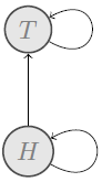
In analogy with the logic G₃, we can refer to the worlds in a Kripke model for G’₃, respectively, as H (Here) and T (There). A Kripke model for G’₃ is a structure like the one shown in Figure 2.

Fig. 2 Kripke model for G’₃

Definition 4. Let M=W,R,v be a Kripke model for G’₃, w ∈ W and φ a formula.

If φ:= p is an atom, we have that: M,w⊨G'3p iff w ∈ v(p).
If φ is not an atom the modeling relation is defined recursively as:

Let φ, ψ be formulas and for all worlds w ∈ W:

(a)M,w⊨G'3φ∧ψ iff M,w⊨G'3φ and M,w⊨G'3ψ,
(b)M,w⊨G'3φ∨ψ iff M,w⊨G'3φ or M,w⊨G'3ψ,
(c)M,w⊨G'3φ→ψ iff for all w' such that wRw', if M,w'⊨G'3φ then M,w'⊨G'3ψ,
(d)M,w⊨G'3¬φ iff there exists w' such that w'Rw,M,w'⊭G'3φ.

We say a formula φ is valid in M and we write M⊨G'3φ, if and only if, for every w ∈ W, M,w⊨G'3φ.

Example 1. Logic G’₃ does not validate the formula p →¬¬ p but it validates the formula ¬¬ p → p.

Proof. Suppose W = {H, T} is the set of worlds, the relation is R = {H, H, H, T, T, T} and lets v_T(p) = 1, and for any other variable and point the valuation is 0, the model is depicted, in the Figure 3. The formula p → ¬¬ p is not valid at H and T in the model. On the other hand, the formula ¬¬ p → p is valid in all Kripke model for G’₃. Indeed, suppose otherwise. Then there is a model such that M,w⊨G'3¬¬p and M,w⊭G'3p for some w∈W. We know that M,w⊨G'3¬¬p, so there is w’∈W for which w’Rw and M,w'⊭G'3¬p and this is, for all w'' ∈ W for which w''Rw' and M,w''⊨G'3p. By the definition of valuation, we must have M,w⊨G'3p, which is a contradiction.

Fig. 3 Kripke countermodel for Example 1

Given the narrow relation between G’₃ and CG’₃, it is natural to think that if there is a Kripke-type semantics for the latter, its semantic must be closely related to that of G’₃.

We can define a type for Kripke semantics to CG’₃ in two different ways. The first based on the semantics of G’₃, and the second redefining the notion of validity as discussed below.

5.1 Semantics-based on G’₃ Semantics

Definition 5. Let M=W,R,v be a Kripke model for G’₃, w ∈ W and φ a formula. We define the modeling relation (denoted by⊨G'3) as follows:

M,w⊨CG'3φ, if and only if there is wRw’ suchM,w'⊨G'3φ.

As we can see, the hereditary property also holds for ⊨CG'3.

Theorem 6. If M,x⊨CG'3φ, and xRy, then M,y⊨CG'3φ.

Proof. The proof is by induction on the length of the formula φ.

The following theorem establishes an equivalence between many-valued semantics and Kripke semantics for CG’₃.

Proposition 2. Let φ be a formula on the language of CG’₃. There exists an interpretation t:L→0,1,2 such that t(φ) = 0, if and only if there is a Kripke model for CG’₃ whose valuation v is such that v(φ) = 0.

Proof. The proof is by induction on the length of the formula φ.

Theorem 7. Let φ be a formula in the language of CG’₃, then:

⊨CG'3φ if and only if for any Kripke model M for CG’₃, it holds that M⊨CG'3φ.

Proof. The proof is by induction on the length of the formula φ and applying Proposition 2.

5.2 Semantics Redefining the Validity Concept

An alternative way of defining the modeling relation for CG’₃ is to consider that the models for CG’₃ are those for G’₃ but changing the Modeling Definition. In ^[²^], the authors explain the notion of being e-valid to the characterization of the validity depends on an existential connective and to distinguish the concept of validity.

Definition 6. A formula φ is said to be e-valid on a model M for logic CG’₃ if exists a point x in M such that M,x⊨CG'3φ.

It is easy to check that this new definition changing the notion of validity coincides with the preceding one.

Lemma 11. Let φ be a formula in the language of CG’₃, then:

⊨CG'3φ if and only if for any Kripke model M for CG’₃, it holds that φ is e-valid.

6 Conclusion and Future Work

Logic CG’₃ was defined in ^[¹³^] utilizing semantics. In this paper, the authors present the logic CG’₃ from a semantic, and syntactic point of view, his contributions are summarized as follows:

A Hilbert type axiomatization for CG’₃ using the Kalmar technique, this axiomatic system satisfies many properties, such as those presented in Theorem 1 and Lemma 1. Among these properties, we can find Deduction theorem, Cut, Rules-AND, among other things. Through this axiomatization, we show that Ł3 and CG’₃ have the same expressive power, Theorem 5.
A characterization of CG’₃ using Kripke models. Thanks to the Kripke semantics for these logics, they obtained a new tool that can help us have a better understanding of paraconsistent logics.

There are some relevant issues associated with the CG’₃ system that needs to be studied. For example, in the semantics approach, there is a many-valued characterization for CG'₃, but an algebraic approach to CG’₃ is still missing. In ^[³^] and ^[⁵^], we can find some algebraic methods such as Blok-Pigozzi and Fidel structures, respectively, that can help the study of these semantics applied to the logic.

Acknowledgments

This work was supported by UNAM-PAPIIT IA105420 and by a postdoctoral fellow grant from Consejo Nacional de Ciencia y Tecnología (CONACYT).

References

1. Anahit, C., Artur, K. (2017). Generalization of Kalmar's proof of deducibility in two valued propositional logic into many valued logic. Pure and Applied Mathematics Journal, Vol. 6, No. 2, pp. 71-75. [ Links ]

2. Borja Macias, V., Perez-Gaspar, M. (2016). Kripke-type semantics for CG’₃. Electronic Notes in Theoretical Computer Science, Vol. 328, pp. 17-29. Tenth Latin American Workshop on Logic/Languages, Algorithms and New Methods of Reasoning (LANMR). [ Links ]

3. Carnielli, W. A., Coniglio, M. E. (2016). Paraconsistent logic: Consistency, Contradiction and Negation; Logic Epistemology, and the Unity of Science Serie 40. Springer: Cham, Switzerland. [ Links ]

4. Chagrov, A. (1997). Modal Logic. Oxford logic guides. Clarendon Press. [ Links ]

5. Coniglio, M. E., Figallo-Orellano, A. (2018). A model-theoretic analysis of Fidel-structures for mbC. In Graham Priest on Dialetheism and Paraconsistency. Springer. [ Links ]

6. Epstein, G. (2017). Multiple-valued logic design: an introduction. Routledge. [ Links ]

7. Ferguson, T. M. (2014). Lukasiewicz negation and many-valued extensions of constructive logics. IEEE 44th International Symposium on Multiple-Valued Logic, pp. 121-127. [ Links ]

8. Galindo, M. O., Macias, V. B., Ramirez, J. R. E. A. (2016). Revisiting da Costa logic. Journal of Applied Logic, Vol. 16, pp. 111-127. [ Links ]

9. Gottwald, S. (2020). Many-valued logic. In Zalta, E. N., editor, The Stanford Encyclopedia of Philosophy. Metaphysics Research Lab, Stanford University, summer 2020 edition. [ Links ]

10. Hájek, P. (2005). Making fuzzy description logic more general. Fuzzy Sets and Systems, Vol. 154, No. 1, pp. 1-15. [ Links ]

11. Ivlev, Y. V. (2013). Generalization of Kalmár's method for quasi-matrix logic. Logical Investigations, Vol. 19, No. 1, pp. 281-307. [ Links ]

12. Mendelson, E. (2009). Introduction to Mathematical Logic. CRC Press. [ Links ]

13. Osorio, M., Carballido, J. L., Zepeda, C., others (2014). Revisiting Z. Notre Dame Journal of Formal Logic, Vol. 55, No. 1, pp. 129-155. [ Links ]

14. Osorio, M., Zepeda, C., Nieves, J. C., Carballido, J. L. (2009). G’3-stable semantics and inconsistency. Computacion y Sistemas, Vol. 13, No. 1, pp. 75-86. [ Links ]

15. Osorio Galindo, M., Carballido Carranza, J. L. (2008). Brief study of G’₃ logic. Journal of Applied Non-Classical Logics, Vol. 18, No. 4, pp. 475-499. [ Links ]

16. Priest, G. (2009). Dualising intuitionictic negation. Principia: an international journal of epistemology, Vol. 13 No. 2 pp. 165-184. [ Links ]

¹ The truth of a compound sentence is obtained by the truth values of its component sentences.

² The valuation v maps the set of propositional variables into the set of truth degrees and can extend to the set of well-formed formulas, as usual.

Received: April 16, 2020; Accepted: February 18, 2021

^* Corresponding author is Everardo Barcenas. ebarcenas@unam.mx

This is an open-access article distributed under the terms of the Creative Commons Attribution License