


 text new page (beta)
 English (pdf)
 Article in xml format
 Article references
 Send this article by e-mail
 Cited by SciELO
  Similars in
SciELO
Similars in
SciELO 
 Permalink
1 Introduction
Nowadays many surveillance systems tend to have multiple interconnected sensors to capture information coming from different modalities (e.g., video and audio). One of the most interesting aspects of current surveillance platforms is their smart capabilities. The idea behind those capabilities is to automate the task of surveillance by means of artificial intelligence algorithms.
For instance, if there is a video-camera, the system should be able to take decisions according to certain events of interest. For example, if the system detects a handgun then triggers the alarm if necessary. Another scenario is to analyze the information from microphones installed on specific places in order to monitor specific commands or even dangerous phrases.
The latter smart capabilities can be achieved by several computer vision and speech recognition strategies. On the one hand, object detection has been used in high resolution cameras installed in specific points of the cities to detect handguns, plates, vehicles, etc. On the other hand, keyword spotting has been integrated in smart devices with multiple microphones such as Amazon Alexa to detect specific events (e.g., glass breaking). Notwithstanding the fact that the performance is acceptable in those cases, there are other valuable scenarios where the performance of these algorithms is unknown. In specific, the effectiveness of state of the art approaches when tested on information coming from devices of common use among people. For example, the audio captured by smartphones or videos of commercial security camera systems.
In this paper, we propose to study and evaluate handgun detection and keyword spotting on information coming from sensors in commercial security systems and smartphones. The idea is to have a study that gives some light about the real performance of the algorithms when using information of common surveillance systems installed in many places in Mexico and typical smartphones. Regarding handgun detection, we are interested in videos from security systems with cameras and internet connection that are configured in houses, stores, or restaurants.
Regarding keyword spotting, we are interested in evaluating the performance to recognize voice commands from audios captured by mobile devices. The idea is to know the performance and viability of integrating handgun detection and keyword spotting in platforms that usually do no have high performance devices to capture video and audio. To the best of our knowledge this is the first time that state of the art algorithms will be studied, adapted and evaluated in the context of Mexico. The main contributions of this paper are as follows:
To build a dataset for handgun detection by using information coming from commercial cameras installed in houses or stores in Mexico.
To build a dataset for keyword spotting of different voice commands in Spanish that were recorded using different mobile devices and capturing different voices that include female and male voices within the age range 18 to 50.
To propose and evaluate a strategy for keyword spotting for recognizing voice commands in audios recorded by smartphones.
To adapt and evaluate state of the art algorithms for handgun detection and tracking in videos.
The rest of this paper is organized as follows. In Section 2 we present the most related work regarding computer vision and speech recognition. In Section 3 and 4, we describe our proposed architecture for Keyword Spotting and the adapted handgun detection strategy respectively. In those sections we also introduce the proposed datasets and the methodology employed to build them. In Section 5, we describe the experiments and evaluation we performed for this work. Finally, Section 6 outlines our main conclusions and future work.
2 Related Work
2.1 Keyword Spotting
Keyword Spotting (KWS) aims at detecting a pre-defined keyword or set of keywords in a continuous stream of audio. In particular, wake-word detection is an increasingly important application of KWS [3]. The solution of this task has been approached by using a wide range of strategies, and in the last years, deep learning methods have dominated the task. For example Arik et al. [1] proposed a Convolutional Recurrent Neural Network (CRNN) approach to solve the Keyword Spotting problem.
This approach uses different CRNN architectures based on Long Short Term Memories (LSTMs) [5] and Gated Recurrent Units (GRUs) [2] architectures that applies convolutions over the mel spectrograms computed from the audio data. The obtained performances are up to 99.6 % of accuracy in a speech dataset.
In other work, an approach proposed by Zhang et al. [15] took advantage of a Deep Stepwhise Separable Convolution Neural Network (DS-CNN) that obtained up to 95.4% in accuracy. The latter accuracy was obtained over the dataset described in [13], which contains one-word audio data pronounced in English. This one-word format for audio data is also used in this work for training the proposed model.
There have been other authors using Separable Convolutions for raw audio data. For example the work described in [8] exploited the mel coefficients and used a SincLayer proposed by Ravinelli et al. [10] for a better feature extraction of the audio data. This model obtained up to 96.4% over the dataset described in [13].
In this work, we propose a model that extracts features from the audio data by computing the mel spectrograms of each audio, but also takes advantage of the use of Deep Stepwise Separable Convolutions for audio classification. As we will show later, our proposed approach can outperform the baselines and reference methodologies.
2.2 Handgun Detection
Handgun detection can be seen as an especial case of the object detection task. The object detection problem has been studied with different approaches. One important aspect in models for object detection is to achieve the highest precision, while reducing the amount of required memory.
In this regard, there have been a number of methods but as well as in keyword spotting, the most outstanding ones have been those that are based on deep learning. For example, the ResNet [4] and ResNetV2 [14] are Residual Networks or ResNets that were first proposed in 2015.
The main aspect of ResNets is to successfully alleviate the vanishing gradient problem, which can impact the network as it becomes deeper in the number of layers.
More recently, there are other popular architectures with promising results, for example; MobilenetV2 [11], YOLOV5 [6] and EffiecientDet [12]. These three networks have the advantage of achieving very high performance with a small computing cost in time and memory compared to previous approaches for the task.
For example, MobilenetV2 is a network designed to run in mobile devices, meanwhile YOLOV5 and EfficientDet are networks that can archive real time detection.
YOLOV5 is currently the state of the art in object detection and is the model that we will adapt and evaluate to make handguns detection. As the experimental evaluation describes by using YOLOV5 we can obtain models with a 65% in gun detection over security cameras images, and acceptable performance to possible fire alerts in videos.
3 Keyword Spotting
The neural network architecture used to recognize audio commands is inspired by previous works described in [8,15,10]. In this paper we propose a novel architecture in order to recognize audio commands in the Spanish language by using a small audio data set to train the model.
In the following sections we describe the methodology to build the dataset, the prepossessing steps to feed the data to the models, and the architecture we designed for this task.
3.1 Dataset
The neural network model proposed for KWS was evaluated in two different datasets. The first dataset corresponds to the one generated in [13], whereas the second dataset was created for this work by manually recording audios from different users and smartphones. The distribution of audios in the generated dataset for training, validation and test is listed in Table 1.
Table 1 Distribution of audios for training, validation and test of the generated dataset
| Training | Testing | Validation |
|---|---|---|
| 928 | 318 | 135 |
As shown in Table 1, the proposed dataset for KWS is composed of 1381 audio files that contain a single audio command with an average duration of 3 seconds per file. The audio files were recorded using mobile devices, then we transform the resulting data into wav files. For this work, female and male voices within the age range 18 to 50 were used to create our dataset. The audio commands recorded in this dataset are predefined as: 'secunet', 'encender', 'apagar' and 'tranquilízate '.
The word 'secunet' is the wake-word that the system is waiting to either execute the command 'encender' or the command 'apagar' and consequently turn the alarm on or off respectively. It is worth to mentiond that the word 'tranquilízate' serves as a wake-word as well as a command and is used to trigger the alarm in a low profile mode using the secret phrase 'tranquilizate tranquilizate' (similar to "take it easy").
Furthermore, there is a negative class 'unknown' that was created using audio files recorded with mobile devices that capture environmental sounds like traffic noises, people talking, etc.
3.1.1 Preprocessing Data
This work aims to detect audio commands from raw wave audio data. However, preprocessing the input data is needed to train and test the proposed neural network architecture. In specific, the input data was standardized using the Python module librosa [7], and reducing the length of each audio to a sequence of size 30,000 data points that represent an average duration of 1 second per audio file. In this case, the start and end points to standardize the audio sequence were randomly chosen in order to create different audio sequences for a single command.
3.1.2 Model Architecture
The architecture of the model used in this work adapts some ideas proposed in [8]. In particular, mel spectrograms are computed for each audio file. This spectrograms are then used as input data of the neural network model. The proposed model consists of four key components.
The first one corresponds to a two dimensional convolutional layer that uses the activation function log(|x| + 1) [8].
The second component is the block of intermediate layers that are in charge of encoding the high discriminative features of the input data.
After this process a Global Average Pooling is applied in order to keep the most salient values of the activation. Finally, the fourth component is formed by dense layers used for audio classification. In the following paragraphs we describe in detail each of this main components.
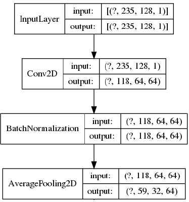
— First convolutional layer: Consists of a two dimensional convolution applied over the mel spectrograms, with the activation function f(x)=log(|x|+1) used in [8]. The structure of this first convolutional layer is described below in Figure 1.
— Intermediate Layers: The intermediate layers of this model are based on the intermediate layers of the Deep Stepwhise Convolutional Neural Network - Short (DS-CNN-S) described in [15]. Each layer consist of a two dimensional separable convolution, with activation function Relu followed by a batch normalization and an Average Pooling with window of size 2 × 2. At the end of the layer a Dropout of probability 0.6 is applied, this avoids over fitting but increases the number of train epochs.
— Global Average Pooling: At the end of the four intermediate layers, a Global Average Pooling is applied to reduce dimension.
— Dense Layers: The dense layers are used to classify the input data in the categories described in 4.2.1.
The model proposed has a total of 56,133 parameters, where 55,493 are trainable and 640 are not. These non trainable parameters correspond to those, which loss function can not optimize using the training data.
4 Handgun Detection
The handgun detection, as mentioned before will be approached by adapting YOLOV5 [6]. In this section we introduce the dataset we built for this task, the adapted model and the parameters used to train the handgun detection model.
4.1 Dataset
In this work we are interested in the task of handgun detection applied to images captured by cameras in real life situations in Mexico. We are also interested in evaluating deep learning models in the state of the art, in particular YOLOV5 [6]. For evaluation purposes we built a new dataset by using information captured from real surveillance systems. We did this by manually crawling images and videos from youtube that represent real life situations in Mexico that show the use of handguns. The majority of this videos show a robbery. This set has 107 positive images (with a gun) and 129 negative images (without a gun). These images will be used to test the model in Section 5.2.
To train the handgun detection model we took advantage of transfer learning. For this purpose the databases from [9] were employed. These datasets are in the YOLO format, which consists in having one xml file for each image that contains the coordinates of the boxes containing all the guns in the image. For our model, we decide to include several types of weapons including knives, but we only evaluate for handgun. We did this way because we hypothesize that different scenarios involving different weapons could share specific contextual visual information useful for the model.
The dataset for guns, [9] has several types of short guns that we included during the training phases. The dataset has also different kinds of knives which were also included in the final model. During the training we use the manual annotations to extract the images intended to be recognized, but also to obtain parts of images that do not contain guns or knifes. This is done in order to reduce the amount of false positives detected by the model. Note that the images in this dataset do not come from security cameras, but they will be used to perform transfer learning and perform hangung detection in the domain of surveillance systems.
4.2 Adapted Model
As previously mentioned the model adapted to perform the handgun detection is a fully convolutional model named YOLOv5 [6]. In contrast to other object detection models, YOLOv5 makes the predictions of the class and position of the object at the same time. This is usually made in separate parts by other works such as RCNNs. This is why YOLOv5 seems to have an advantage over the other models when we are making object detection on low resolution images, where the steps for detection an track are learned at the same time.
It is worth to mention that YOLOv5 has 4 different sizes. The difference between these model sizes is the number of convolutional layers employed. For this research work we used the medium model. In specific this model was trained with the dataset described in Section 4.1.
The data described there was splitted into 80% for training and 20% for test. We trained the model during 300 epochs.
5 Results
5.1 Key Word Spotting Results
The model of Keyword Spotting proposed in this work was evaluated using the collected data set described in Section 3.1. To evaluate the effectiveness of the proposed model, we use the accuracy, the F1 score, the precision and recall metrics.
We compare this model with a DS-CNN model proposed by [15], an LSTM based convolutional model described in [1], a model using just two simple dimensional convolutions, and a model that uses an adaptation of the model proposed in [8], which uses the mel coefficients instead of the mel spectrograms used in this work. The confusion matrices for each training are also presented as comparison of the different evaluated models in this work.
In the next subsections we present each of the models used for comparison. We performed the evaluation training with the different datasets described above and the performance obtained by using the metrics presented in the last paragraph.
5.1.1 Evaluation of the Proposed Model
The purpose of this experiment is to observe the performance of the proposed model in a dataset of real life instances collected by users and their smartphones. This model was trained with 5000 epochs using a batch size of 100 samples. After training the model, the confusion matrix obtained by evaluating the model over the test set are presented in tables below. The x axis of the confusion matrix corresponds to the predictions made by the model, whereas the y axis corresponds to the labels of the corresponding audio files. The order of appearance of the audio commands for this dataset is 'ambiente', 'apagar', 'encender', 'tranquilízate ', 'secunet'.
This classes are represented in the confusion matrix using the shortenings 'amb', 'ap', 'enc', 'tran' and 'sec' respectively.
The results shown in Table 2 prove that the proposed model have outstanding performance. For this experiment the overall accuracy is 83.01% over the test set and 88.14% over the validation set. The accuracy and F1 score by class is presented in Table 3 and the average metrics in Table 4.
Table 2 Confusion matrix of the proposed model
| Confusion matrix | |||||
|---|---|---|---|---|---|
| amb | ap | enc | tran | sec | |
| amb | 35 | 3 | 1 | 0 | 0 |
| ap | 0 | 51 | 3 | 3 | 3 |
| enc | 2 | 1 | 59 | 2 | 6 |
| tran | 1 | 3 | 2 | 57 | 7 |
| sec | 0 | 2 | 8 | 7 | 62 |
Table 3 Metrics by class for the proposed model
| Metrics by class | ||||
|---|---|---|---|---|
| accuracy | precision | recall | f1-score | |
| amb | 0.978 | 0.90 | 0.92 | 0.91 |
| ap | 0.9334 | 0.85 | 0.85 | 0.85 |
| enc | 0.9214 | 0.84 | 0.81 | 0.83 |
| tran | 0.9214 | 0.81 | 0.83 | 0.82 |
| sec | 0.8962 | 0.78 | 0.79 | 0.79 |
5.1.2 Evaluation of Simple Convolutional Model
The aim of this experiment is to compare the performance of this specific architecture. This model was also trained with 5000 epochs and a batch size of 100. The results presented in Table 5 show that the model reached an overall accuracy of 76.72% over the test set. Over the validation set the model obtained an accuracy of 76.73%
Table 5 Confusion matrix of the model created using simple convolution layers
| Confusion matrix | |||||
|---|---|---|---|---|---|
| amb | ap | enc | tran | sec | |
| amb | 38 | 0 | 1 | 0 | 0 |
| ap | 3 | 47 | 4 | 4 | 2 |
| enc | 1 | 0 | 61 | 4 | 4 |
| tran | 1 | 6 | 10 | 46 | 7 |
| sec | 5 | 5 | 10 | 7 | 52 |
The metrics by class are presented in Table 6 and one can appreciate that the results obtained by the proposed model outperforms this Simple Convolutional model by several points in different metrics. In Table 7 we present the average metrics for this model, which is lower than the obtained results of our proposal in Table 4.
Table 6 Metrics by class of the simple convolutional model
| Metrics by class | ||||
|---|---|---|---|---|
| accuracy | precision | recall | f1-score | |
| amb | 0.9654 | 0.97 | 0.79 | 0.87 |
| ap | 0.9245 | 0.78 | 0.81 | 0.80 |
| enc | 0.8931 | 0.87 | 0.71 | 0.78 |
| tran | 0.8774 | 0.66 | 0.75 | 0.70 |
| sec | 0.8742 | 0.66 | 0.80 | 0.72 |
5.1.3 Evaluation of Convolutional Long Short Term Memory Neural Network (CLSTMNN)
The aim of this experiment is to compare the performance of the Convolutional Long Short Term Memory Neural Network (CLSTMNN). For this we present the results obtained from a model that uses Long Short Term Memory neural networks after applying a convolutional layer over the mel sprectrograms. The confusion matrix of this model is presented in Table 8.
Table 8 Confusion matrix of the model using CLSTMNN.
| Confusion matrix | |||||
|---|---|---|---|---|---|
| amb | ap | enc | tran | sec | |
| amb | 36 | 1 | 0 | 2 | 0 |
| ap | 4 | 47 | 0 | 1 | 8 |
| enc | 2 | 1 | 28 | 21 | 18 |
| tran | 0 | 3 | 8 | 36 | 23 |
| sec | 4 | 8 | 12 | 7 | 48 |
The metrics by class are presented in Table 9 and the average metrics are presented in Table 10. From these tables we see that an accuracy of 61.32% was obtained using this model over the the test set, the same accuracy score was obtained over the validation set. These results are notably lower than the previous models that we have evaluated at this point.
Table 9 Metrics by class of of the CLSTMNN model
| Metrics by class | ||||
|---|---|---|---|---|
| accuracy | precision | recall | f1-score | |
| amb | 0.9591 | 0.92 | 0.78 | 0.85 |
| ap | 0.9182 | 0.78 | 0.78 | 0.78 |
| enc | 0.805 | 0.40 | 0.58 | 0.47 |
| tran | 0.7956 | 0.51 | 0.54 | 0.53 |
| sec | 0.7484 | 0.61 | 0.49 | 0.55 |
5.1.4 Deep Stepwhise Separable Convolutions Model
The purpose of this experiment is to compare the performance of the Deep Stepwhise Separable Convolutions. For this, we trained a model based on [15] that also uses separable convolutions, this model was trained in 4500 epochs with a batch size of 100. In Table 11 we present the confusion matrix obtained by training this model with the specific settings we already described. The metrics by class of this model are presented in Table 12, whereas the average metrics are presented in Table 13. From these results we can observe that this method is our closest competitor in performance. We hypothesizes that the combination for Convolutions and the recurrent information in the network are playing a key role for capturing discriminative information.
Table 11 Confusion matrix of the Deep Stepwhise Separable Convolutions model
| Confusion matrix | |||||
|---|---|---|---|---|---|
| amb | ap | enc | tran | sec | |
| amb | 38 | 1 | 0 | 0 | 0 |
| ap | 0 | 49 | 1 | 3 | 7 |
| enc | 4 | 3 | 56 | 2 | 5 |
| tran | 1 | 4 | 3 | 52 | 10 |
| sec | 3 | 4 | 4 | 3 | 65 |
Table 12 Metrics by class of of the Deep Stepwhise Separable Convolutions Model
| Metrics by class | ||||
|---|---|---|---|---|
| accuracy | precision | recall | f1-score | |
| amb | 0.9717 | 0.97 | 0.83 | 0.89 |
| ap | 0.9277 | 0.82 | 0.80 | 0.81 |
| enc | 0.9308 | 0.80 | 0.88 | 0.84 |
| tran | 0.9182 | 0.74 | 0.87 | 0.80 |
| sec | 0.8868 | 0.82 | 0.75 | 0.78 |
5.1.5 Model using the Mel Coeficients
In this final experiment for Keyword Spotting, we are interested in observing the overall performance of other traditional features employed in Speech Recognition for this task. Thus, in this section we present the results obtained from the model that uses the mel coefficients instead of the mel spectrogram of the audio, a similar idea was presented in [8]. This model was trained with 4500 epochs and a batch size of 100. The confusion matrix of the predictions is presented in Table 14. From Table 14 we see that an overall accuracy of 77.24% was obtained. The metrics by class are presented in Table 15, whereas the average metrics are presented in Table 16.
Table 14 Confusion matrix of the model created using mel coefficients
| Confusion matrix | |||||
|---|---|---|---|---|---|
| amb | ap | enc | tran | sec | |
| amb | 37 | 0 | 1 | 0 | 1 |
| ap | 0 | 48 | 3 | 4 | 5 |
| enc | 0 | 1 | 63 | 2 | 4 |
| tran | 1 | 3 | 4 | 52 | 10 |
| sec | 4 | 6 | 6 | 7 | 56 |
Table 15 Metrics by class of the simple convolutional model
| Metrics by class | ||||
|---|---|---|---|---|
| accuracy | precision | recall | f1-score | |
| amb | 0.978 | 0.95 | 0.88 | 0.91 |
| ap | 0.9308 | 0.80 | 0.83 | 0.81 |
| enc | 0.934 | 0.90 | 0.82 | 0.86 |
| tran | 0.9025 | 0.90 | 0.82 | 0.77 |
| sec | 0.8648 | 0.71 | 0.74 | 0.72 |
Table 16 Average metrics of the model using mel coeficients
| Average metrics | |||
|---|---|---|---|
| Accuracy | f1 score | Recall | Precision |
| 0.80503 | 0.81544 | 0.8200 | 0.8127 |
Based on the results presented in the tables above, we can compare the different performance of the models evaluated in Table 17. In this table we can observe the different accuracy values obtained for the different models over the test set. From these results we have empirical evidence that the proposed model achieve the best results for the task of Keyword Spotting in the studied domain. In specific for the task of identify commands in audios collected by users that used their smartphones.
5.2.1 Evaluation for Image Classification
The aim of this experiment is to evaluate the performance of the adapted YOLOv5 architecture to predict if there is a handgun in images coming from commercial security cameras.
For this purpose we used the dataset described in Section 4.1 into an image classification setting. To measure the performance of the algorithm, we have created a framework to evaluate the performance in gun detection.
Thus, we will evaluate this adapted YOLOv5 by using the final score in the prediction as a probability threshold to determine the final class.
We can see from Tables 18 and 19 that if the probability threshold is reduced, the accuracy and the F1-scores improves, but the number of false positive predictions increase, but the false negatives decrease.
Table 18 F1-Scoreforthe hand gun class and accuracy of YOLOv5 detecting images with a handgun using different probability thresholds. The dash denotes that there were not any positive prediction
| pt/Metric | F1-score | Accuracy |
|---|---|---|
| 0.8 | — | 54.47% |
| 0.6 | 7.21% | 56.17% |
| 0.4 | 15.13% | 57.02% |
| 0.2 | 24.42% | 57.87% |
| 0.1 | 39.74% | 61.28% |
| 0.05 | 49.71% | 62.13% |
| 0.01 | 64.66% | 65.11% |
Table 19 Confusion matrices of detection of images with a hand gun. These are the results using different probability thresholds with YOLOv5
| pt | Positive | Negative | |
|---|---|---|---|
| 0.8 | Pos pred Neg pred |
0 107 |
0 128 |
| 0.6 | Pos pred Neg pred |
4 103 |
0 128 |
| 0.4 | Pos pred Neg pred |
9 98 |
3 125 |
| 0.2 | Pos pred Neg pred |
16 91 |
8 120 |
| 0.1 | Pos pred Neg pred |
30 77 |
14 114 |
| 0.05 | Pos pred Neg pred |
44 63 |
26 102 |
| 0.01 | Pos pred Neg pred |
75 32 |
50 78 |
This is an important parameter to determine when the security system is implemented, since a false positive and false negatives might have different consequences, depending on the application.
The specific way we use the probability threshold pt for each result is as follows: the test images will be label as 0 and 1, where 1 means that the image has a gun and 0 that the image does not have a gun.
With these labels, we compute the Confusion matrix, Accuracy and F1-score.
5.2.2 Evaluation for Object Detection
This model is intended to detect where the gun is inside the image. This is the reason why the following metrics shall be interesting. As we mentioned in Section 4.1, we have the annotations of the images containing a "box" which shows where the gun is in the image. In this case, we are only interested on testing using the images from the test set that have a gun in them. With these images we will compute the following metrics:
— Predicted boxes: total of predicted boxes in all the images from the test set.
— Real boxes: total number of boxes in the annotations.
— Intersected boxes: total of predicted boxes that intersect at least one real box.
As in Section 5.2.1, we will only consider the boxes with a probability greater than a given threshold pt. The evaluation was conducted using pt ∈ {0.8, 0.6, 0.4, 0.2, 0.1, 0.05, 0.01}. The results obtained are shown in Table 20. As we can see, we have a low number of intersection between boxes. If we use a high probability threshold, there are few handguns detected but these detection tend to be accurate. As we reduce the prediction threshold, the number of intersected boxes is improved, but the accuracy in the detection is affected. The results in Section 5.2.1 can be used to determine the best probability threshold for each application.
Table 20 The results of the object detection in the test set using YOLOv5. It shows the number of predicted boxes, number of real boxes and number of intersected boxes, using different probability thresholds.
| pt/Metric | Predicted | Real | Intersected |
|---|---|---|---|
| 0.8 | 0 | 108 | 0 |
| 0.6 | 4 | 108 | 4 |
| 0.4 | 9 | 108 | 12 |
| 0.2 | 15 | 108 | 24 |
| 0.1 | 25 | 108 | 44 |
| 0.05 | 36 | 108 | 70 |
| 0.01 | 74 | 108 | 125 |
5.3 Evaluation for Video Detection
The purpose of this experiment is to evaluate the proposed strategy for handgun detection in videos. The algorithms was evaluated in five different videos from security cameras of the collected dataset. All the videos have a duration of approximately 30 seconds. For this evaluation, we take 3 frames per second and make the detection. The results from these experiments are shown in Table 21.
Table 21 Results from the algorithm in 5 videos and all the different confidence thresholds used. It shows the results of accuracy, F1-score, intersected boxes and detected boxes. The dash denotes that there were not any positive prediction
| Video | pt | Acc. | F1 | Intersec. | Detec. |
|---|---|---|---|---|---|
| Video 1 | 0.8 | 34.44% | — | 0 | 0 |
| 0.6 | 34.44% | — | 0 | 0 | |
| 0.4 | 41.11% | 18.46% | 6 | 6 | |
| 0.2 | 55.55% | 68.25% | 16 | 67 | |
| 0.1 | 61.11% | 75.52% | 26 | 84 | |
| 0.05 | 63.33% | 77.55% | 34 | 88 | |
| 0.01 | 65.55% | 79.19% | 70 | 90 | |
| Video 2 | 0.8 | 5.48% | — | 0 | 0 |
| 0.6 | 5.48% | — | 0 | 0 | |
| 0.4 | 6.85% | 2.86% | 1 | 1 | |
| 0.2 | 9.59% | 8.33% | 2 | 3 | |
| 0.1 | 17.81% | 25% | 6 | 11 | |
| 0.05 | 41.10% | 55.67% | 13 | 28 | |
| 0.01 | 84.93% | 91.85% | 34 | 66 | |
| Video 3 | 0.8 | 64.77% | — | 0 | 0 |
| 0.6 | 64.77% | — | 0 | 0 | |
| 0.4 | 65.91% | 6.25% | 0 | 1 | |
| 0.2 | 69.32% | 40% | 0 | 14 | |
| 0.1 | 65.91% | 46.42% | 1 | 25 | |
| 0.05 | 69.32% | 60.87% | 1 | 38 | |
| 0.01 | 50% | 56.86% | 2 | 71 | |
| Video 4 | 0.8 | 15.91% | — | 0 | 0 |
| 0.6 | 15.91% | — | 0 | 0 | |
| 0.4 | 18.18% | 5.26% | 2 | 2 | |
| 0.2 | 27.27% | 37.25% | 10 | 28 | |
| 0.1 | 44.32% | 59.50% | 20 | 47 | |
| 0.05 | 79.54% | 88.46% | 26 | 82 | |
| 0.01 | 84.09% | 91.36% | 48 | 88 | |
| Video 5 | 0.8 | 84.27% | — | 0 | 0 |
| 0.6 | 84.27% | — | 0 | 0 | |
| 0.4 | 88.76% | 44.44% | 4 | 4 | |
| 0.2 | 86.52% | 40% | 4 | 6 | |
| 0.1 | 82.02% | 33.33% | 5 | 10 | |
| 0.05 | 67.42% | 21.62% | 8 | 23 | |
| 0.01 | 49.44% | 21.05% | 12 | 43 |
As we can see, the confidence threshold of 0.4 seems to be the one with the best performance in video. This is because it has a low number of false positives. Also it made some accurate predictions when it detects something. In video, we should give more weight to the false positives, since we will analyze 3 frames per second, this leads to have false positives that are more expensive than false negatives.
6 Conclusion and Future Work
In this paper we built a dataset for Keyword Spotting in Spanish and Handgun detection. We evaluate the performance of adapted versions of methods in the state of the art and showed their performances under different scenarios. These tasks are aimed to be useful in real life situations where there are installed commercial surveillance systems.
The idea is to have a study that shows the performance of state of the art methodologies that can complement security platforms of commercial systems. The motivation of this is that most of the time, the evaluation of object detection and keyword spotting are made on data collected by devices that are not available for most people in countries like Mexico. The experimental results in this paper, showed that the proposed architecture for Keyword Spotting is an alternative for this task achieving performances above 83% in accuracy. Regarding handgun detection, the adapted methods can be used if we are able to determine the specific threshold that benefits the domain.

