


 text new page (beta)
 English (pdf)
 Article in xml format
 Article references
 Send this article by e-mail
 Cited by SciELO
  Similars in
SciELO
Similars in
SciELO 
 Permalink
1 Introduction
The continuous signals discretization must meet accuracy specifications; these are often ignored. The sampling frequency is essential; the well-known sampling theorem is fundamental, but not sufficient. These specifications are very remarkable in calculating the signal peak-values; mainly when the research is conducted on a small-scale. Therefore, the acquired digital information quality is an essential descriptor for all measurement and control systems.
It is desirable to choose a sampling frequency that does not represent a heavy burden for the data acquisition system. In many applications, this sampling rate implies an efficient use of the central processing unit or data acquisition hardware. On the other hand, the sampling rate to acquire, save and transmit less information can be reduced and then interpolate in the receiver [1].
Shannon's sampling theorem [2, 3] establishes the minimum angular sampling frequency
For instance, a sinusoidal signal
For the abovementioned, mathematical expressions are necessary for a relationship between the sampling rate and the measurement accuracy. However, there are some practical criteria. For instance, for control systems, the sampling frequency should be based on knowledge of their characteristics. Thus, it is reasonable to consider the closed-loop control system bandwidth, or the rising time [4]. A good selection takes the sampling frequency between 10 and 20 times greater than the bandwidth.
Automatic control systems have dynamic characteristics of low-pass filters, allowing a relatively low sampling frequency, among other aspects of their designs [5]. The relations abovementioned can be small for typical signal processing applications [1, 6], [7].
A practical criterion for sea wave [8, 9] is to consider the signal spectrum peak frequency
All the above cases are based on practical criteria guaranteeing an acceptable accuracy depending on the application type. However, when an application should not increase the computational cost in real-time or the data acquisition card does not allow a higher data sampling rate, there are other solutions.
For example, If the application provides post-processing of collected data, several methods can be applied to reduce sampling frequency's adverse effect without increasing it so much. This paper intends to be useful for the academy, researchers and industry. It is possible to calculate the maximum error due to sampling frequency based on mathematical expressions. A comprehensive general analysis is developed based on the relation between the sampling frequency and the maximum measurement error for a sinusoidal signal. The harmonic of greater amplitude is relevant in many applications and computation types [10–24]].
As mentioned previously, the sinusoidal signals type is the basis for finding the proposed formulations by this paper in Section 2. Besides, they have been used in various applications developed successfully for several years. Those mathematical expressions are useful in signals with several harmonics if their objective-bandwidth is well-thought-out; or otherwise, those that have some significant harmonics. In this sense, Section 4 will analyze several experimental examples where the previous statements are true.
The paper's remainder has several sections: Review; Material and Methods; Experimentations and Results, which present signals for a wave generation hydraulic channel and biomechanical signal measurements in Parkinson disease patients; Discussion and Conclusions.
2 Review
A physically modelled process, such as a wave research laboratory for maritime and coastal works design, requires calculating the signals' peak values [8, 9, 22, 25], as Fig. 1 shows.
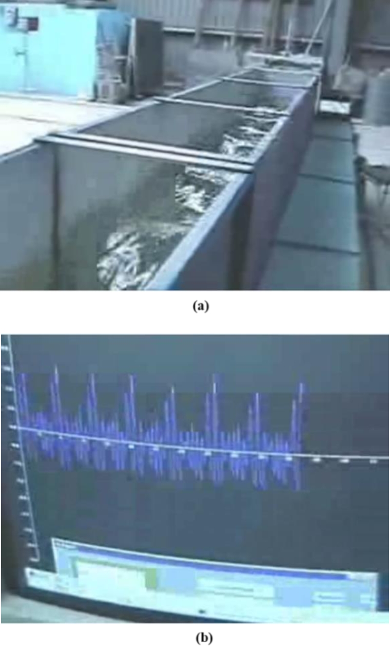
Fig. 1 Wave research laboratory for maritime and coastal works designs: a) Rectangular section measuring channel; b) Signals with relevant peak-values
Assessments use small-scale models, and their computations are transformed into real-scales, finally. Maximum errors must be calculated with high accuracy in the laboratory to know and evaluate their real-works impacts.
Similar situations occur in the design of mechanical systems [26]. In other measurement systems, for example, in biomechanical assessments, the multiple freedom degrees of their triaxial signals and wireless communication bandwidth limitations may not allow increasing the sampling rate, as shown in Fig. 2. In these cases, signals' peak-values computations are relevant. This known behaviour enables us to give the appropriate treatment to acquired signals and obtain good results in the advanced digital signals processing and when artificial intelligence methods are used [18–21, 27]].

2 Material and Methods
2.1 Measurement Accuracy and Sampling Frequency
This section presents several analyzes and examples that improve understanding of the relationship between sampling frequency and measurement accuracy for signals composited of several harmonics. This analysis is based on the bandwidth and the error expressions for a sinusoidal signal, in real-time and post-processing mode, which is useful when a designer must present with absolute certainty the accuracy specifications of a measurement system being very relevant when the signal peak-values are calculated.
2.2 Data Post-Processing Mode
Real-time calculations are not necessary for many applications. Instead, these computations can be made on data previously acquired (post-processing mode) to calculate the maximum and minimum signal values. Fig. 3. Presents the absolute maximum error due to sampling frequency during the peak-value calculation

Where
Replacing
The relative maximum error
2.3 Real-Time Processing Mode
The absolute maximum error in real-time is located symmetrically to coordinate axis origin, where the highest signal change speed occurs, as shown in Fig. 4. The maximum error is calculated using a zero-order hold. Therefore, a signal sample remains valid until the next sample is taken (next sampling period):
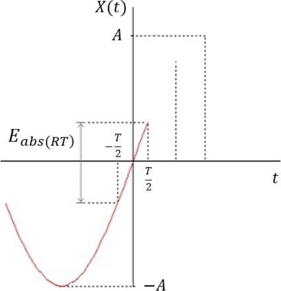
Fig. 4 The absolute maximum error in real-time measurements for a sinusoidal signal with frequency f
where
where
The maximum relative error in real-time
Fig. 5 shows the illustration of the absolute maximum error produced around the peak values in real-time processing mode
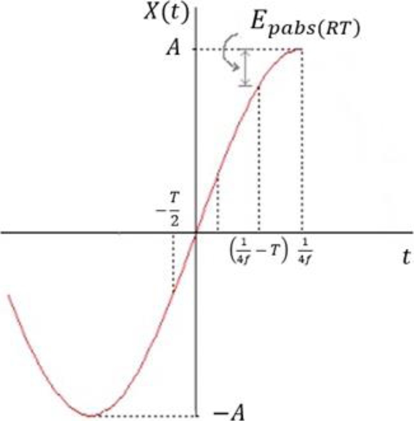
Fig. 5 The absolute maximum error produced around the peak values in real-time processing mode
The sampling period can be written as
Equation (27) shows the relative maximum error in real-time, regarding the peak-to-peak of signal value
Table 1 presents the results of the evaluation of the Eqs. (10), (19) and (28) for several sampling frequencies, being
Table 1 Relative errors and sampling frequency
| n |
|
|
|
| 2 | 50 | 100 | 100 |
| 4 | 14.64 | 50 | 70.71 |
| 8 | 3.8 | 14.64 | 38.26 |
| 10 | 2.44 | 9.54 | 30.9 |
| 20 | 0.61 | 2.44 | 15.64 |
| 50 | 0.098 | 0.39 | 6.27 |
| 100 | 0.024 | 0.098 | 3.14 |
| 200 | 0.0061 | 0.024 | 1.57 |
| 300 | 0.0027 | 0.0109 | 1.04 |
|
| |||
3 Experimentations and Results
3.1 Wave Generation Hydraulic Channel
Fig. 6 presents a typical signal for a wave generation hydraulic channel used at physical modelling on time and frequency domains, in post-processing mode for a segment between 17 to 26 seconds. This signal harmonics are less than 1.1 Hz, and it was sampled at 192 and 4 samples per second, simultaneously. There is a significant loss of information around the maximum peak value with a sampling frequency of 4 Hz. Nevertheless, the maximum error during the peak-value calculation in post-processing mode has not occurred because the red signal points are not equidistant from the peak-value. If the sampling frequency of 192 Hz is considered as reference, Eqs. (20) and (30) present the relative error (𝑒𝑝𝑟𝑒𝑙(𝑃𝑂𝑆)) produced around the peak-values in post-processing mode, in per cent. In maritime hydraulics for small-scale physical modelling, those errors are substantial.
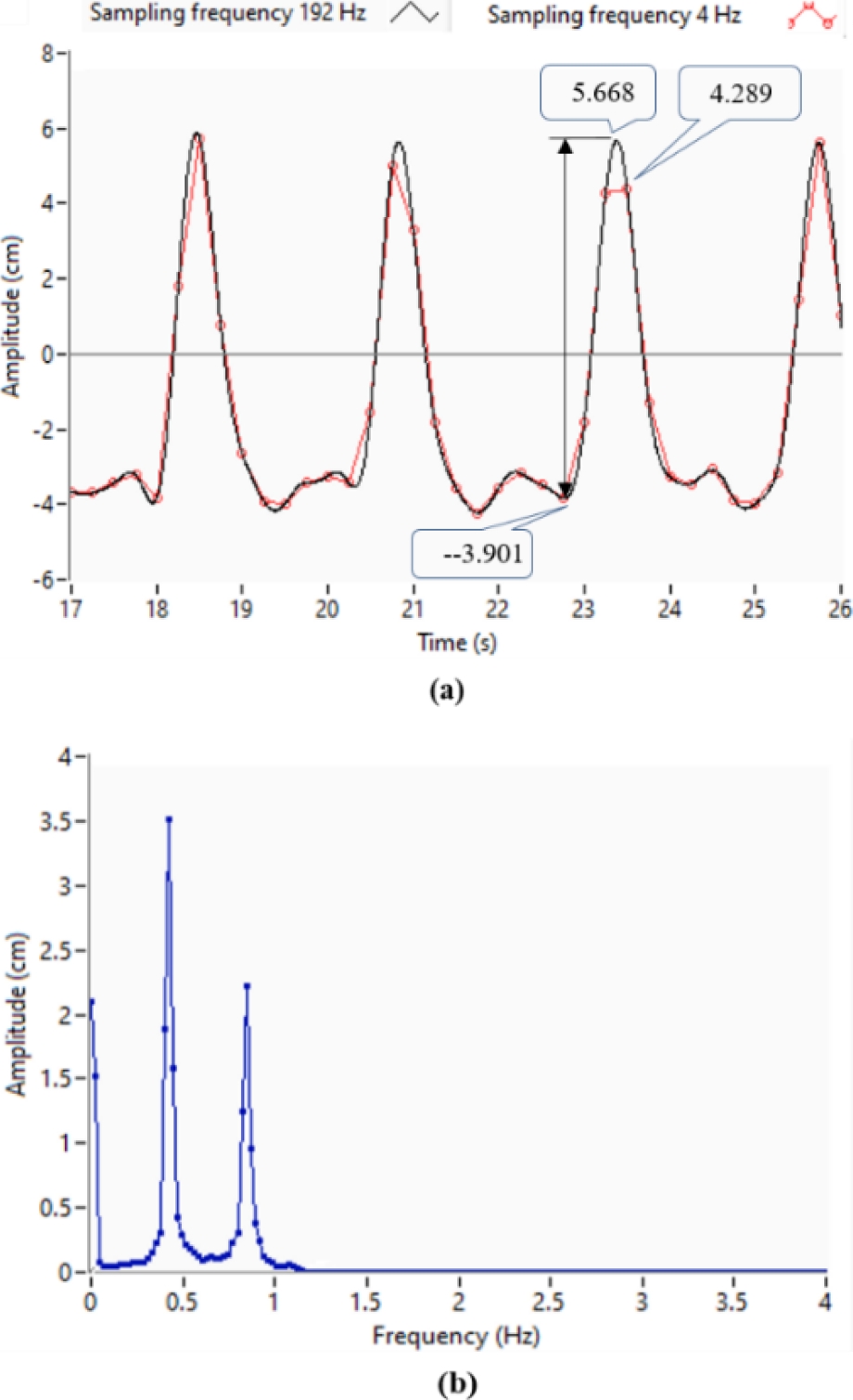
Fig. 6 A typical signal for a wave generation hydraulic channel: a) The time-domain signal with 192 Hz and 4 Hz sampling frequency; b) The frequency domain signal sampled at 192 samples per second. The highest frequency harmonic is 1.1 Hz
In this example, the behaviour was less severe because there is only an error during the maximum peak computation and one sample coincided with the minimum peak. Eq. (30) presents the relative error produced around the peak value in post-processing mode, in per cent, for a signal segment between 22 and 24 seconds:
The relative maximum error
3.2 Biomechanical Signal Measurement in Parkinson Disease Patients
In this application, the hardware and communication devices are not allowed to use a higher sampling frequency. The three inertial measurement units with nine degrees of freedom (accelerometer, gyroscope and magnetometer tri-axial) are connected to a computer by Bluetooth, and there is limited bandwidth.
Fig. 7 presents a left-hand postural tremor of a Parkinson disease patient with a sampling frequency of 50 Hz (50 samples per second). Fig. 7c shows the peak amplitude spectrum. This signal has been sampled five times concerning the highest-frequency harmonic, which is 10 Hz. Based on Eq. (10), the relative maximum error
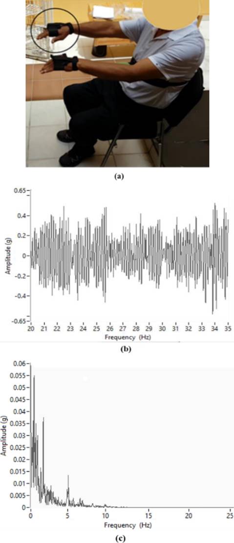
Fig. 7 A left-hand postural tremor: (a) A Parkinson disease patient; (b) Y-axis signal of the accelerometer; (c) Magnitude spectral (peak). The highest frequency-harmonic is 10 Hz
Fig. 8 presents a signal section of Fig. 7b from 31.5 to 32 seconds with a sampling frequency of 300 Hz (reference) and 50 Hz, respectively (simultaneous sampling) with test hardware. Eq. (32) presents a relative error produced around the peak value in post-processing mode in per cent for the segment mentioned above.

Based on Eq. (10) the relative maximum error
The relative error
A measurement system's maximum error specification means that the measurement error will not be greater than the worst-case scenario's specified maximum error. In the examples shown, that statement is true. In numerous cases analyzed, the behaviour is similar, and it can be stated that the formulations proposed have a very favourable practical value.
4. Discussion
Eqs. (10), (19) and (28) present the relative errors according to the sampling frequency for a sinusoidal signal. However, for composed signals of several harmonics can be considered its bandwidth or the highest-frequency harmonic. In other words, the frequency range in which most of the signal power is concentrated. For example, in Fig. 7c the harmonics with frequencies greater than 10 have very small amplitudes and minimum energy. For instance, in Fig. 7c the harmonics with frequencies greater than 10 have very small amplitudes and therefore, a minimum power.
The Eq. (10) is useful because the relative error
In many cases, when hardware limitations do not allow increasing the sampling frequency, the cubic spline interpolation is a good option [18, 21]. In several applications, a practical criterion is to use an interpolation factor from 5 to 10. Interpolation factor greater than ten does not offer appreciable improvements. Fig. 9a presents a signal section of Fig. 7b with a sampling frequency of 50 Hz, with cubic spline interpolation factor equal to 1 (equivalent sample rate of 100 Hz) for a time interval from 11.5 to 12 seconds. Fig 10b another time interval from 33.5 to 34 seconds. In both cases, the cubic spline interpolation effect enables greater accuracy in peak-values calculations, decreasing the error due to the sampling frequency.
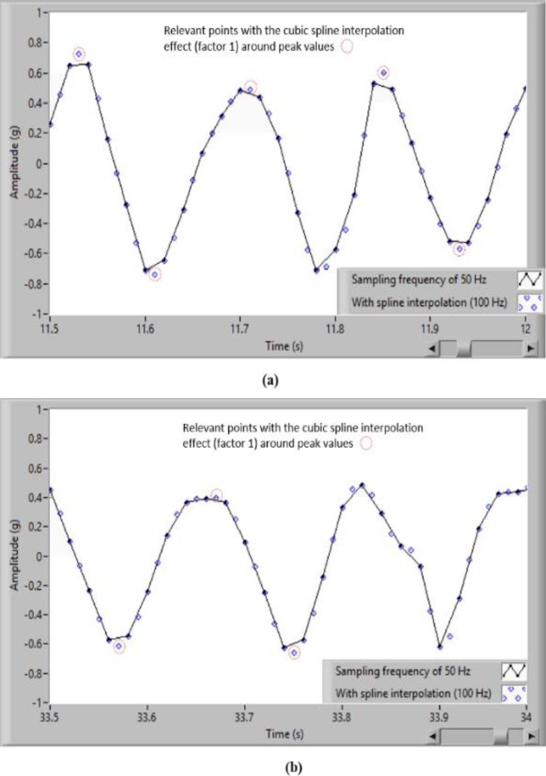
Fig. 9 A signal section of Fig. 7b with a sampling frequency of 50 Hz, with cubic spline interpolation factor equal to 1 (equivalent sample rate of 100 Hz); a) A time interval from 31.5 to 32 seconds; b) Another time interval from 33.5 to 34 seconds
4.1 Comparison with some Works more Closely Related
Often, measurement errors due to the sampling frequency are not quantified. If not possible to increase the sampling frequency, some methods to reduce its effect on the measurement accuracy must be used. Generally, few works analyze in a practical way or present mathematical expressions of the error due to the sampling rate, especially in peak-values calculations. This section presents a comparison with some work more closely related.
Paper [22] only evaluates the measurement error in wave research laboratories, fundamentally, based on a sinusoidal signal. That work presents one graph of the cubic spline interpolation and does not quantify its effect on the raw signal.
The paper [28] examines the impact of digital processing, and discretization or sampling of sea surface elevations. The theory of random linear waves, the probability distributions for the measured wave heights and amplitudes have been obtained as conditional for the sampling frequency. Rates of 1 Hz or less may lead to significant underestimation of the probability of huge waves.
In [29] and [25] the relationship between the sampling frequency and measurement's maximum error is obtained for continuous sinusoidal signals The data are processed using the Fast Fourier Transform (FFT) and interpolation of cubic splines. Graphical and statistical examples are shown for a wave research laboratory.
The paper [30] presents the phase-locked spikes in various types of neurons encode temporal information. The metric called vector strength (VS) quantifies the degree of phase-locking. In electrophysiological experiments, the timing of an action potential is detected with finite temporal precision, which is determined by the sampling frequency. The errors in VS, assuming random sampling effects will be estimated. The impacts of analogue-to-digital conversion (ADC) quantization noise on the recovery of harmonic amplitudes and phases in the presence of large fundamental amplitudes are examined by theory and simulation [30], to determine the noise limits of instrumentation system design for power systems monitoring and harmonic power-flow measurement.
In this paper, a comprehensive analysis is developed based on the relation between the sampling frequency and the maximum measurement error for a sinusoidal signal. The real-time processing mode presents mathematical expressions of relative maximum errors around the peak-values. The relative maximum error of peak-values calculation in post-processing mode is analyzed with more relevance. Additionally, signals composited of several harmonics have some illustrative examples.
Biomechanical signals and research laboratories waves are objectives of this work as interesting examples. The error due to sampling frequency is quantified in a material very understandable. Some examples evaluate the cubic spline interpolation and its effects. Besides, the general analysis is useful for any signal where the peak-values computation represents the main aim. For many years, the research group has used these design criteria to evaluate several data acquisition systems' performance based on sampling frequency. For examples, for wave research and hydraulic laboratories [23, 31]; environmental noise in urban areas and airports [12–16]]; biomechanical signal analyzes [18–21, 32]]; and fault diagnose based on mechanical vibrations [33, 34].
5 Conclusions
The Eq. (10) allows calculating the relative maximum error produced around the peak-values in post-processing mode. Eq. (19) computations the relative maximum error in real-time. Likewise, Eq. (28) is the representations of the error around the peak-values also in real-time. These three equations have utility in signals with several harmonics if their objective-bandwidth is well-thought-out; or otherwise, signals that have some significant harmonics. Many applications have demonstrated the usefulness of these design criteria to evaluate the data acquisition systems' performance. These equations permit to quantify the measurement accuracy based on sampling frequency. The error by samples rate always will be less than the maximum error computed by these equations. The maximum relative mistake during the peak-values calculation in post-processing mode is analyzed with more relevance because it is widely used in many engineering areas.
The cubic splines interpolation, widely mentioned and well-accepted by many authors and available in signal-processing commercial software, reconstructs the time-series adding intermediate points, producing an effect that could be considered similar at a higher sample rate. A practical criterion in several applications is to use an interpolation factor from 5 to 10. In general, the interpolation factor greater than ten does not offer appreciable improvements.

