


 text new page (beta)
 English (pdf)
 Article in xml format
 Article references
 Send this article by e-mail
 Cited by SciELO
  Similars in
SciELO
Similars in
SciELO 
 Permalink
1 Introduction
The objective of this study is the creation of a forecasting model for the workload in the maintenance industry. We will briefly introduce the industry to better contextualize the motivation behind the study and the significance of having an accurate forecast.
The maintenance industry operates the maintenance of commercial facilities. It provides services of repairs and maintenance of various nature (electrical, plumbing, mechanical, drainage, fabric) that require different skills. The customer can request these services in a planned maintenance contract, quoted work, reactive tasks, and emergency tasks. A planned maintenance contract is where the work is scheduled to take place on a regular basis.
This contract agrees for a number of visits per month to the facilities for regular maintenance. Quoted work is where by customer initiative or by engineer advice after a visit, a repair or renovation is requested that requires budgeting and customer approval. Reactive and Emergency work is when a repair of some urgency is required (ie. lights are out). The general workflow of this industry consists of an operations team that is based on an office and a mobile workforce of engineers and subcontractors of flexible size.
The operations team is responsible for the creation and assignment of tasks. The engineer’s team is responsible for traveling to each store to execute the repairs.
1.1 Motivation
The planned work is assigned by the operation team to the individual engineers, with some margin left for emergency calls that can occur on a daily basis. In the past this has been done based on employee experience, this study pretends to partly automate the process and improve efficiency.
Depending on the workload there may be a need to plan for extra hours, to hire more engineers or subcontractors, or to reduce the number of tasks per engineer. A poor forecast will create risks by excess workload per engineer if the forecast is lower than the actual workload. While if the forecast is too high the operations team allocates too many resources causing financial loss. An accurate forecasting of the workload is essential to find the right balance of efficient staffing without creating risks by overworking employees.
In this paper, we will look at the data that has been captured of a company operating in the maintenance industry. We will look at the characteristics of the data and what steps have been taken to pre-process it. We will show the data analysis and draw conclusions about its characteristics and the challenges it presents.
We start by looking at related work previously done. Then we do a data analysis and how we handled the data pre-processing. We discuss the Evaluation metric chosen, and finally look at the implementation of forecasting models for this time series.
2 Related Work
Time series forecasting is a problem that has been studied for a long time with applications in multiple areas [1]. We find studies in many areas such as patient workload [10], sales forecasting [3], call centers call volume [2], energy consumption [7], and many more. The approaches vary, with some approaches taking a univariable approach [11] where the forecast is based only on previous values. And approaches that use additional data to complement the time series like using multiple related time series [3] to train the forecasting model.
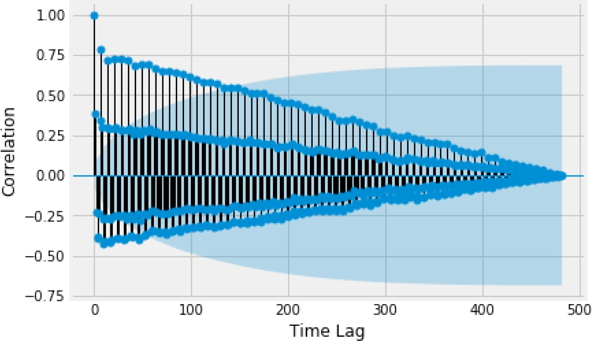
In this initial study, we will focus on a univariable approach since there is a strong correlation in the dataset with its past values (Fig. 2 ) and there are no other time series in the database that correlate to the workload.

3 Data
The data that we used for analysis in this study was created in a proprietary cloud application and stored in a SQL database.
The platform has a web/desktop environment that the operations team uses to create tasks for each customer. The platform is operating for over a year and it contains 483 days of data. In our study we are interested in the task workload so we focused on the Tasks table. From this table we selected the date start and date end fields that capture the beginning and ending time of a task (see table 1). There are 18593 tasks completed in this dataset corresponding to the work done over 483 days.
Table 1 Tasks table
| task_id | date_start | date_end |
| ... | ... | ... |
| 24107 | 2019-05-29 10:28:32.070 | 2019-05-29 12:11:27.287 |
| 24158 | 2019-05-29 12:44:11.470 | 2019-05-29 13:39:04.697 |
| ... | ... | ... |
3.1 Data Preprocessing
The data for this study comes from a production SQL database. From the database, we obtain a list of all completed tasks. For the purpose of this study, we need to transform this data into a fixed step time series. After retrieving the list of tasks we start by removing those tasks that have null dates or are outside the data range studied.
While some of these may have a wrong date due to user error, with null or invalid dates it is impossible to know to what day they correspond so these tasks are dropped from the dataset. Then we calculate each task duration based on the start date and completion date timestamps. Examining the calculated task’s duration we see that there are some oddities in the dataset. The minimum task duration is under -153 days and the maximum over 365 days. Given the nature of the data, we know these outliers to be impossible since all tasks are completed on the same day.
These errors are due to user input error. For every task with zero duration, negative duration, and duration over 10 hours, we assume that the duration is invalid. Then we impute the task duration with the mean task duration. This is an important step, because removing the tasks would cause a drop in the corresponding day’s workload value and provide a lower forecast. Finally, we sum the task’s duration per day using a rolling window of one day to obtain the total daily workload.
3.2 Data Analysis
Plotting the daily workload reveals some interesting characteristics of the dataset (Fig. 1).
There is a clear weekly cycle, with the workload dropping drastically on the weekends. There is a big drop at the end of December, this matches the Christmas Holiday season. So clearly weekends and holidays have an influence on the workload value. We can also notice that there is some variance from month to month. This hints at some yearly seasonality to the workload. Plotting the autocorrelation with different time lags (Fig. 2).
This plot shows the correlation between an observation at time t and the observations at t-0,t-1,..,t-n. We can observe that there is some correlation with past values at fixed time steps. The strongest correlation is with the previous week (7 day time lag) as can be seen in Fig. 2. So incorporating this behavior into the model will likely result in a better forecast. We can also see how the correlation value decreases the further back in time we look.
4 Evaluation Metric
To evaluate the quality of the model we must first decide on a metric. For this experiment we are interested in how close the forecasted value is to the real value, so we will need to measure the difference between forecast and ground truth and minimize the error. In regression models we can find a few good options such as MAE (Mean Absolute Error), MSE (Mean Square Error), RMSE (Root Mean Square Error) and MAPE (Mean Absolute Percentage Error).
For our study, RMSE was the metric of choice. Since it results in a value in the same unit as the values being measured it provides an intuitive understanding of the results. And by taking the root square of the error, larger errors have a bigger influence on the reported value so big deviations from the actual value will be punished in the result.
The MAE and MSE erros values are not in the same units as the dataset making it less intuitive. The MAPE [9] presents its error value in a percentage value that has the advantage of being scale independent [6]. But MAPE encounters issues that results in a division by zero error [8] in data sets where the values reach zero, as is the case with the dataset of this study.
Root Mean Square Error (RMSE) Root Mean Square Error is perhaps the most commonly used metric to evaluate forecasting errors. Its formula is similar to MSE, but by taking the square root of the MSE value it presents the error in the same units as the values, making it intuitive to interpret the results:
5 Forecasting Models
For our experiment, we divided a dataset into a training set and a test set, using a 70% / 30% split. Due to the sequential nature of a time series, the last 30% are used as the test set.
5.1 Persistence Model
To establish a baseline we start with a simple persistence model. This model takes the last value on the time series and uses it as the forecast (Fig. 3). This model obtains an error (RMSE) of 71.37 hours. This is a very high error for a dataset where the mean daily workload is of 89.79 hours.
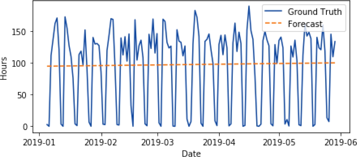
5.2 Linear Regression
Linear regression is a classical statistical model, easily understandable but somewhat limited. Linear regression can be used for time series forecasting. For our study it proves insufficient to capture the complex nature of this dataset. Nonetheless, the linear regression model reveals the general trend of the dataset.
As we can see in (Fig. 4), this model fits poorly to the dataset, failing to account for the weekly cycle. It obtains an error (RMSE) of 62.92 hours, but it shows some an improvement over our baseline.
5.3 Linear Regression + Seasonal Model
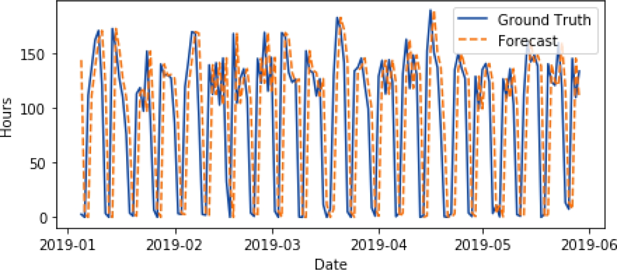
Time series can be decomposed into several components such as level, trend, seasonality and noise [4, 5]. In our study, we use the linear regression model as our trend and de-trend the dataset. Using the now stationary dataset, we create a model to handle the seasonality.
We use a least-squares polynomial fit with a cycle of 7 days, since this value displayed the highest correlation (Fig. 2). Combining the Linear Regression model and the Seasonal Model results in a much better forecast for our dataset (Fig. 5) with an error (RMSE) of 25.96 hours. This method effectively handles the trend of the dataset and the seasonality.

5.4 Residual Data
If we subtract the trend model and the seasonality model from the original time series we obtain the residual data (Fig. 6).

This difference reveals the data that is not captured is this forecasting model and that accounts for the error values. Further work will explore how this data can be used to further improve the forecast results.
6 Conclusion and Future Work
This study revealed some of the challenges and limitations. But it also reveals some avenues to be explored.
Simple models like linear regression are not sufficient to obtain an accurate forecast since they can not handle seasonality. But combining Linear Regression with the week cycle model significantly improved accuracy. The method has its limitations, such as not being able to handle more complex trends.
Further work will be done by exploring other models. While the proposed method does a good job of handling trend and seasonality in this dataset, there is residual data (Fig. 6) that is unused. Exploring methods that take advantage of the residual data could further improve the results.
This study focused on univariable forecasting, but likely augmenting the data with additional information (weekends, holidays, seasons) will likely improve the accuracy so further work could explore models capable of handling multivariable forecasting.

