


 text new page (beta)
 English (pdf)
 Article in xml format
 Article references
 Send this article by e-mail
 Cited by SciELO
  Similars in
SciELO
Similars in
SciELO 
 Permalink
1 Introduction
The task of grouping a set of objects in a cluster where the objects inside are more similar to each other in the same cluster (group) than objects in other clusters is called Cluster Analysis or Clustering, the cluster analysis is one of most important research areas at present, as a part of data science or data mining, clustering is used in many fields like pattern recognition, machine learning and image analysis.
A main task of Data Mining is to process the natural language, the cluster analysis is essential in the natural language processing, today exists many algorithms built to make the hard work of grouping texts more accurate and efficient, is essential to make a comparison of the algorithms in order to know the strengths and weaknesses of each of them. Is important to know that notion of a ”cluster” cannot be precisely defined, which is one of the reasons why there are so many clustering algorithms [2].
There is a common denominator: a group of data objects. However, different researchers employ different cluster models, and for each of these cluster models again different algorithms can be given. The notion of a cluster, as found by different algorithms, varies significantly in its properties.
Understanding these ”cluster models” is the key to understand the differences between the various algorithms.
2 Related Work
Due to the large number of existing clustering algorithms, experimental evaluations in specific fields are useful, in this case, the tests were focused on the Natural Language Processing field.
There are some interesting papers that made a comparison of different clustering algorithms applied to Document Clustering, in [11] a comparison between Agglomerative and Partitional algorithms is made, in this paper the better results were obtained by partitional algorithms, and agglomerative clustering algorithms performs the worst results, the partitional algorithm used in [11] was K-Means, and was tested in a very large dataset.
On the other hand, in [10] the authors made a comparison between Bisecting K-Means, Regular K-Means and UPGMA in Hierarchical clustering, in this case the better results were obtained by Bisecting K-Means, followed by Regular K-Means, and the worse were the agglomerative hierarchical method UPGMA.
A more complete comparison is made in paper [9], where K-Means, Heuristic K-Means and Fuzzy C-Means were compared, the interesting point of this paper is that the authors use different pre-processing methods in texts, like tf-idf, tf and boolean representation schemes, in summary Heuristic K-Means obtained the best results, followed by K-Means, the best results in the paper comes from the combination of a partitional algorithm, tf.idf and making a stemming before cluster the documents.
This previous works evaluate algorithms with different procedures on the clustering process, algorithms from different categories and a compar-ison of the obtained results when using different methods in the pre-clustering process. Based on this works, this paper will show the outputs of three different partitional algorithms (the best in consulted literature), preparing texts with tf.idf and stemming.
3 Data Clustering Algorithms
This section presents a taxonomy of the different approaches to clustering algorithms as well as the theoretical explanation of each clustering algorithm used in this paper.
3.1 Taxonomy of Clustering Algorithms
Actually, there are so many clustering algorithms, and each one of them has different applications and characteristics, also, this algorithms can be categorized focusing on the technical details of the general procedures of the clustering process, a graphic representation of this categories is shown below (Fig. 1). An explanation of this taxonomy is [3]:
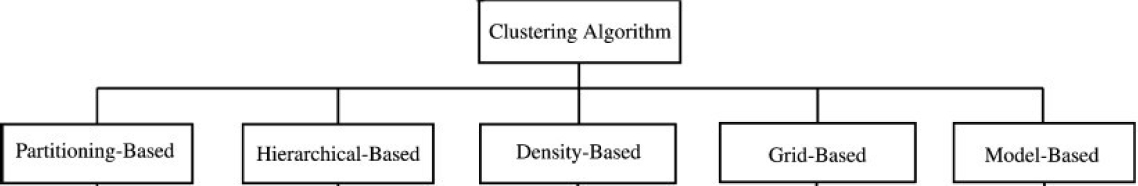
— Partitioning-Based: In this kind of algorithms, clusters are determined promptly, the partitioning algorithms divide the data into a partitions, where each partition represent a cluster. In this algorithms each cluster must contain at least one object, and each object must belong to exactly one group.
— Hierarchical-Based: This methods can be agglomerative or divisive, both organize the data in a hierarchical way. The dataset is represented by a dendrogram, where individual data is presented by leaf nodes.
— Density-Based: In this algorithms, elements are separated based on their regions of density, connectivity and boundary. They are closely related to point-nearest neighbors. A cluster is defined as a group of elements considered as neighbors depending of their density as a group, and grows in any direction that density leads to.
— Grid-Based: The space of the data objects is divided into grids. The accumulated grid-data make grid-based clustering techniques independent of the number of data objects that employ a uniform grid to collect regional statistical data, and then perform the clustering on the grid, instead of the database directly.
— Model-Based: Such a method optimizes the fit between the given data and some (predefined) mathematical model. It is based on the assumption that the data is generated by a mixture of underlying probability distributions.
The three algorithms to be analyzed on this paper belongs to Partitioning-Based category.
3.2 Affinity Propagation
Affinity Propagation forms clusters by sending messages between pairs of instances until convergence and considers all data points as potential exemplars, this algorithm can determine the number of clusters by itself unlike K-Means or Spectral Clustering.
The algorithm proceeds by sending messages in two steps, between two matrices
[2]: a R matrix called
“responsibility matrix”, with
where responsibility matrix updates are sent around and (2), (3) are the way to update the availability matrix:
for
Once the cluster boundaries stop changing over a number of iterations, the
algorithm extracts the exemplars and clusters from the final matrices as those
whose “responsibility + availability” be positive, (i.e
3.3 K-Means
This algorithm was first proposed by Stuart Lloyd in 1957 [6]. K-Means uses vector quantization methods in order to get a partitioning of the data space into Voronoi cells returned as clusters. K-Means commonly uses a random initial points called “seeds” and then proceeds by alternating between two steps to select new cluster centroids.
The partitioning of the observations according to the Voronoi diagram generated by the means, is calculated as:
where 4 must be fulfilled
Calculating the new centroids within the new clusters is realized with the following equation:
The algorithm has converged when assignments stop changing, that means what the Voronoi cells(clusters) are complete. The use of heuristic algorithms implies that the results could not be the optimum.
3.4 Spectral Clustering
Spectral Clustering algorithm uses the eigenvalues of a similarity matrix obtained from the data, to realize dimensionality reduction and then it makes clustering in less dimensions. The similarity matrix passed as a parameter to the algorithm gives a quantitative assessment of the similarity of each par of points in the data, like an adjacency matrix used for graphs.
Spectral Clustering works on relevant eigen-vector of a Laplacian Matrix of A, this algorithm project the data into a lower-dimensional space (the eigenvector domain) where they are easily separable with other methods like K-Means, once the dimensionality reduction is complete, the process for cluster the data in this lower-dimensional space is the same that K-Means.
4 Weighting and Measuring Methods
This section presents the followed processes to achieve the preprocessing, weighting and measuring the similarity of the texts.
4.1 The Weighting TF-IDF Algorithm
The Term Frequency - Inverse Document Frequency (TF-IDF) [5] is a numerical statistic that is intended to reflect how important a word is to a document in a collection or corpus [8]. This method weights the words in a text or a set of texts, the TF-IDF value increases proportionally to the number of a word appears in the corpus, with this quantization of the words, can be created a mathematical model of each text in the corpus. A word that appears a lot of times in the corpus is less important for the texts than word that appears just a few times in the corpus, which is more important for TF-IDF is the product of the following two statistics:
1. Term Frequency: Is calculated by counting the times that a term appears in a text (raw frequency), for better results can be used the “Augmented Frequency”, this is the raw frequency of a term divided by the raw frequency of the most occurring term in document, and is described as follow:
2. Inverse Document Frequency: It is obtained by dividing the total number of documents by the number of documents containing the term, and then taking the logarithm of that quotient, this process is called “logarithmically scaled inverse fraction”, and is described as follow:
In this equation
Once the algorithm have obtained the Term Frequency and the Inverse Document Frequency, the TF-IDF values are the product of the Term Frequency values and the Inverse Document Frequency values, this operation is calculated as:
In TF-IDF a high weight describe a very important term, and a low weight describe a less important term, when TF-IDF is complete, a mathematical form of each text is available.
4.2 The Cosine Similarity Measure
Cosine Similarity is a similarity measure between two non-zero vectors that uses
cosine of the angle between this vectors, taking into consideration that the
In data clustering, the cosine similarity is commonly used to know how similar two documents are, in this field, each term is notionally assigned a different dimension and a document is a vector where the value in each dimension corresponds to the number of times the term appears in the document. With two vectors of attributes, A and B, the cosine similarity use a dot product and magnitude as:
where
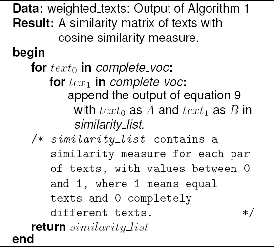
Once the cosine similarity was already calculated for each par of texts in corpus, the similarity matrix of texts is complete, this matrix gives the similarity measure of each text with each text.
5 Preparing the Corpus
5.1 Tokenizing and Stemming Texts
Assuming
The
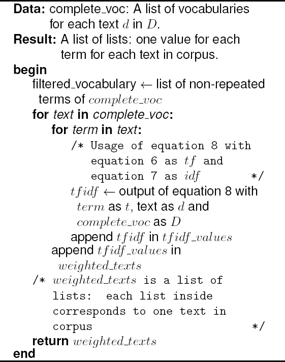
5.2 Weighting Terms and Texts with TF-IDF
Once the texts have been processed and standardized, is necessary to obtain the
weights (relevance) for each word in the corpus
The output of the tf-idf algorithm will be used to build the similarity matrix using the cosine similarity method. See the Algorithm 1.
5.3 Building the Similarity Matrix using Cosine Similarity
To build a similarity matrix of the corpus
6 Clustering the Texts
The algorithms to be tested were described in 3.2, 3.3 and 3.4, a very complete implementation of each algorithm is available in the scikit-learnfn Python library, specifically the sklearn.cluster classfn, the test were realized in this implementations by sending the matrices obtained with the previous algorithms as parameters. Each implementation has a set of customizable options that can help to improve the results.
6.1 Clustering with Affinity Propagation
The Affinity Propagation algorithm is interesting because of its
ability to obtain the number of clusters by itself based on the data, as
described in 3.2. Complexity is the main drawback of Affinity
Propagation, well this one has a complexity of the order
Affinity Propagation is effective when: exists many clusters, when there is an uneven cluster size, the data is in a non-flat geometry or for a unknown number of clusters.
6.2 Clustering with K-Means
K-Means unlike Affinity Propagation, needs a defined number of clusters as a parameter, this is why will be used the number of clusters obtained by Affinity Propagation, this increases the autonomy of the tests by avoiding the human intervention and gives a more computer-made clusters.
K-Meanscan be used effectively when: there is an even cluster size, the data is in a flat geometry or there are too many clusters, the accuracy of K-Means when converging in the optimum will depends on the initial centroids, which are randomly selected.
For this tests, the initial centroids will be determined by k-means++ [1] algorithm, the n-clusters will be the Affinity Propagation n-clusters, to increase de accuracy, the algorithm will be run 300 times with different centroid seeds, the results will be the best output of this consecutive runs.
6.3 Clustering with Spectral Clustering
Spectral Clustering as explained in 3.4, does a low-dimension embedding of the affinity matrix between samples, followed by a K-Means in the low dimensional space. Spectral Clustering like K-Means, requires the number of clusters to be specified, this n clusters will be the Affinity Propagation n-clusters to avoid the human intervention, for improve the results, once the dimensionality reduction is complete, K-Means will be run 100 times with different centroid seeds. This algorithm is useful when: there are few clusters, there is an even cluster size or the data is in a non-flat geometry.
7 Evaluation of the Algorithms
7.1 The Corpus
The supervised corpus was taken from the PANfn, which consists in 60 problems, each problem contains 20 texts and have the gold standard. Each algorithm’s set of clusters will be compared with the supervised corpus, the tables will have 3 columns: corpus is a set of 20 texts, ground truth with the expected results and the algorithm column, with the obtained set of clusters.
The structure of each set of clusters is the following: Cluster x :
[text_a, text_b, ...,
text_c] where
Which indicates how many relevant items are selected, and an f-measure value which is the harmonic mean that combines the precision and recall values [7], in this 3 averages, a score of 1 means that the algorithm-made clusters are exactly equal to the supervised corpus and 0 score means that they are completely different. Although the proposed method works for any corpus and was tested in more than sixteen different corpus, for illustrative purposes each table will contain the comparison of 2 corpus with their respective set of clusters both supervised and algorithm-made.
7.2 Affinity Propagation Clusters
Table 1 contains two comparison examples of the Affinity Propagation clusters with the supervised corpus and their respective execution time, precision average, recall average and f-measure average.
Table 1 Affinity Propagation algorithm evaluation table
| Corpus | Ground truth | Affinity Propagation clusters |
| 1 | n_clusters: 5 Cluster 1 : [7] Cluster 2 : [8, 9, 10, 11, 14, 15, 16, 19, 20] Cluster 3 : [2, 4, 5, 6, 12, 13] Cluster 4 : [3] Cluster 5 : [1, 17, 18] |
n_clusters : 5 Cluster 1 : [2, 3, 4, 6, 7] Cluster 2 : [5, 8, 11, 19, 20] Cluster 3 : [9, 13, 16] Cluster 4 : [10, 12, 14, 15] Cluster 5 : [1, 17, 18] Execution time: 0.1387 seconds Precision average: 0.750 Recall average: 0.554 f-measure average: 0.624 |
| 2 | n_clusters: 5 Cluster 1 : [5, 7, 19] Cluster 2 : [1, 4, 14, 20] Cluster 3 : [10, 11] Cluster 4 : [3, 6, 15, 16] Cluster 5 : [2, 8, 9, 12, 13, 17, 18] |
n_clusters: 5 Cluster 1 : [1, 3, 4, 5, 6, 14, 20] Cluster 2 : [2, 8, 9, 13, 15, 17] Cluster 3 : [7, 10, 11] Cluster 4 : [12, 16, 18] Cluster 5 : [19] Execution time: 0.1589 seconds Precision average: 0.678 Recall average: 0.658 f-measure average: 0.616 |
7.3 K-Means Clusters
Table 2 contains two comparison examples of the K-Means clusters with supervised corpus and their respective execution time, precision average, recall average and f-measure average.
Table 2 K-Means algorithm evaluation table
| Corpus | Ground truth | K-Means clusters |
| 1 | n_clusters: 5 Cluster 1 : [7] Cluster 2 : [8, 9, 10, 11, 14, 15, 16, 19, 20] Cluster 3 : [2, 4, 5, 6, 12, 13] Cluster 4 : [3] Cluster 5 : [1, 17, 18] |
n_clusters : 5 Cluster 1 : [10, 12, 14, 15] Cluster 2 : [5, 8, 11, 19, 20] Cluster 3 : [9, 13, 16] Cluster 4 : [1, 17, 18] Cluster 5 : [2, 3, 4, 6, 7] Execution time: 0.2784 seconds Precision average: 0.576 Recall average: 0.720 f-measure average: 0.616 |
| 2 | n_clusters: 5 Cluster 1 : [5, 7, 19] Cluster 2 : [1, 4, 14, 20] Cluster 3 : [10, 11] Cluster 4 : [3, 6, 15, 16] Cluster 5 : [2, 8, 9, 12, 13, 17, 18] |
n_clusters: 5 Cluster 1 : [1, 3, 4, 14, 16, 20] Cluster 2 : [10, 11, 19] Cluster 3 : [5, 7] Cluster 4 : [2, 6, 9, 12, 15, 17, 18] Cluster 5 : [8, 13] Execution time: 0.4063 seconds Precision average: 0.663 Recall average: 0.774 f-measure average: 0.615 |
7.4 Spectral Clustering Clusters
Table 3 contains two comparison examples of the Spectral Clustering clusters with the supervised corpus and their respective execution time, precision average, recall average and f-measure average.
Table 3 Spectral Clustering algorithm evaluation table
| Corpus | Ground truth | Spectral Clustering clusters |
| 1 | n_clusters: 5 made Cluster 1 : [7] Cluster 2 : [8, 9, 10, 11, 14, 15, 16, 19, 20] Cluster 3 : [2, 4, 5, 6, 12, 13] Cluster 4 : [3] Cluster 5 : [1, 17, 18] |
n_clusters : 5 Cluster 1 : [2, 6, 8, 9, 11, 12, 13, 19, 20] Cluster 2 : [3, 4, 7] Cluster 3 : [1, 17, 18] Cluster 4 : [10, 14, 15] Cluster 5 : [5, 16] Execution time: 0.2949 seconds Precision average: 0.532 Recall average: 0.844 f-measure average: 0.556 |
| 2 | n_clusters: 5 Cluster 1 : [5, 7, 19] Cluster 2 : [1, 4, 14, 20] Cluster 3 : [10, 11] Cluster 4 : [3, 6, 15, 16] Cluster 5 : [2, 8, 9, 12, 13, 17, 18] |
n_clusters: 5 Cluster 1 : [1, 4, 14, 16, 20] Cluster 2 : [8, 9, 12, 13, 17] Cluster 3 : [10, 11] Cluster 4 : [2, 3, 6, 15, 18, 19] Cluster 5 : [5, 7] Execution time: 0.3463 seconds Precision average: 0.867 Recall average: 0.823 f-measure average: 0.822 |
8 Results
As it is shown on the results of the performed tests, the most efficient algorithm in time terms was Affinity Propagation which complete the clustering with a time average of 0.148 seconds, next was Spectral Clustering with a time average of 0.317 seconds, and K-Means was the worst on time terms with a time average of 0.342 seconds.
On the other hand there are the precision, recall and F-measure averages, in Precision terms the better average was obtained by Affinity Propagation with 0.704 of precision, the second was Spectral Clustering with an score of 0.694, and the worst was K-Means with an average of 0.619, in recall terms, Spectral Clustering obtained a 0.833 score, the next was K-Means with an average of 0.747, the last was Affinity Propagation which obtained a 0.606 score, finally the better F-measure average was obtained by Spectral Clustering with an score of 0.758, the next was K-Means with an average of 0.677, at the end was Affinity Propagation with an average score of 0.651, this is showed in Table 4, where the Spectral clustering algorithm has the best result.
9 Conclusion and Future Work
While Affinity Propagation had the best precision average, Spectral Clustering had the highest recall and F-measure averages, being K-Means the worst of the three algorithms. In this paper the algorithms were tested with small datasets, possibly this is a reason why Spectral Clustering got the best results because it works better with few clusters while Affinity Propagation works better with many clusters and large datasetsfn. K-Means uses heuristic algorithms to converge in a possible local optimum, which can cause poorly results depending on the initial random seeds that K-Means choose, even if K-Means works well with few clusters. K-Means works with flat geometry while Spectral Clustering and Affinity Propagation works with non-flat geometry, due to the nature of the data and the probabilistic nature of how words are distributed, any two documents may share many of the same words [10], theoretically with the non-flat geometry of documents Spectral Clustering and Affinity Propagation must have given the best results, but is important to remember that the size of the tested datasets wasn’t the appropriate for Affinity Propagation.
Finally is important to analyze why Spectral Clustering was the best in F-measure average; this algorithm realize a dimensionality reduction using the eigenvectors of the similarity matrix before clustering in fewer dimensions (converting the data into a flat geometry), this gives to the K-Means phase of Spectral Clustering a compressed version of the dataset but without loss of information, practically, Spectral Clustering transform a non-flat geometry into a flat geometry that is the appropriate for K-Means algorithm.
The experimental evaluation of the algorithms, shows that for small datasets with a non-flat geometry Spectral Clustering gives the best results in comparison with K-Means or Affinity Propagation however is important to remember that Affinity Propagation calculate the number of clusters by itself unlike the other two algorithms, in the tests both Spectral Clustering and Affinity Propagation gave good results, obviously those results were conditioned to the nature of the analyzed datasets (size, distribution, number of terms, etcetera). Spectral Clustering works well with few clusters and responds well to a non-flat geometries, better that K-Means with a previous dimensionality reduction.

