


 text new page (beta)
 English (pdf)
 Article in xml format
 Article references
 Send this article by e-mail
 Cited by SciELO
  Similars in
SciELO
Similars in
SciELO 
 Permalink
1 Introduction
Throughout their lives, it is estimated that one in eight women [7] will suffer from breast carcinoma, of which approximately 80% will be ductal carcinomas. Likewise, one in nine men suffers from prostate carcinoma.
Early detection is aimed at identifying the disease when it has not yet acquired infiltrating character, and is limited to the glandular ducts (in situ), without having infiltrated the glandular parenchyma yet.
At this point, the disease can only be eradicated with surgery that removes the affected duct segment, plus a disease-free safety margin, preserving the rest of the patient's breast, with a success rate greater than 90%.
In the case of prostate carcinomas, the specific prostate antigen, which has traditionally been used as a tumour marker, has proved to be imprecise for the screening of men for the disease. In both cases, it is of great interest to characterize the disease when it is still in situ, and for this, computational simulation can be an excellent tool to investigate it.
Carcinogenesis is a phenomenon in which one or multiple mutations in certain genes allow cells to reproduce and survive abnormally, under a selection process that leads to uncontrolled tumor growth of an infiltrating nature. There are many mathematical models in the literature [1,2,3,5,8,9,11] that incorporate the knowledge we currently have about the genes involved in these neoplasms, and that study the mutations they undergo to end up giving rise to a CIS. In this paper, we propose a CIS model that uses a simulation based on a three-dimensional cellular automaton to model a generic glandular duct, and analyze how the mutations in the cells of the simulated duct become CIS.
We also apply the model on known data of intraductal breast adenocarcinoma, parallelize it, and study its natural history with the parallel model and the acceleration achieved.
2 Biology of CIS
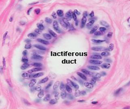
In a healthy human gland [2], the excretory ducts have a cylindrical morphology and are responsible for the secretion that the gland secretes (milk during lactation, or prostatic fluid).
These ducts, with a cross-sectional structure made up of two layers of cells (Figure 3); the innermost layer is called the luminal layer, and the outermost layer that surrounds it is called the myoepithelial layer. The entire package is wrapped in a basal membrane.
Luminal cells are known to reproduce frequently throughout life, in response to the endocrine estrogen-progesterone axis for the breast, or the testosterone axis in the prostate. During cell reproduction, in the process of copying the genetic load, mutations can accumulate in the areas of the genome that control the processes of cell survival and reproduction. Ductal adenocarcinomas usually originate in the luminal cells and have an in situ character when they grow through the light of the tumour, without surpassing the basement membrane or infiltrating the glandular parenchyma that contains the duct. In the case of the human breast, it is currently known that the two types of cells that form the ducts have their origin in a single class of progenitor cell which, by means of cellular differentiation, gives rise to two germinal lines that conclude in the two aforementioned cell types.
Continuing the analysis in the case of the human breast, Figure 1 illustrates the process of cell differentiation that results in a mature pipeline from stem-type progenitor cells, according to the currently published literature. As can be seen, stem cells are differentiated into two subtypes of germinal progenitor cells that end up differentiating into the two cell lines that form the duct, with the luminal cells in the light of the duct, and with a layer of myoepital cells between these and the basement membrane. This differentiation is determined by the cellular microenvironment, and by the presence of certain growth factors.
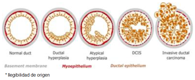
Fig. 1 Natural history of adenocarcinomas in situ, and their transformation into infiltrating adenocarcinomas from a normal duct (left) to a carcinoma in situ
In the model this aspects will be determined by a set of probabilities chosen ad hoc, so that a pipeline of physiological initial conditions is obtained. It is also known that women with a genetic predisposition to breast cancer accumulate inherited mutations that make them more prone to contracting the disease, estimating the number of cases due to this circumstance to be up to 12%.
Without prejudice to other genes that may be involved in the pathogenesis of the disease, it is currently known that mutations in the BRCA1, BRCA2, PTEN and TP53 genes increase the probability of suffering a ductal carcinoma. In the model, this genetic predisposition will be taken into account by means of a logical HMG variable.
In our simulation, the stem cells of the duct will be defined with the genetic predisposition incorporated in the genome of all of them.
The meaning of the four genes we will consider in the simulation is illustrated in tables 1 and 2.
Tabla 1 Genes involved in CIS pathogenesis
| Gene | Normal Expression |
|---|---|
| BRCA1 | Allows the cell a normal work |
| BRCA2 | Allows mitosis |
| PTEN | Activates cellular apoptosis when there are malignant mutations Inhibits cells neoplastic reproduction |
| TP53 | Apoptosis in case of proto-oncogene damage Apoptosis if alterations architecture of double layer |
Tabla 2 Genes involved in CIS pathogenesis and their expression when mutated
| Gene | Pathological Expression |
|---|---|
| BRCA1 | Cellular Death |
| BRCA2 | Allows uncontrolled mitosis |
| PTEN | Does not activate apoptosis if there are malignant mutations Does not inhibit neoplastic reproduction |
| TP53 | Celll survives eve with damage in their proto-oncogenes The cell survives even with alterations in the double-layer architecture |
In them, the first and second columns collect the modelled genes and their functioning under physiological conditions. When one or more of the genes are damaged, the behaviour of the host cell becomes malignant.
When a particular chain of mutations leads to In particular, malignant transformation is consolidated not only when there is a mutation in the BRCA2 gene, but it is a multifactorial process [16] that also requires that cell safety mechanisms, which are regulated by the tumour suppression genes (PTEN) and programmed cell death or apoptosis (TP53), also fail. In this situation, the natural history of the clone of cells that host it leads inexorably to the proliferation of ductal carcinoma, first in situ, and then infiltrating when this clone breaks the duct and expands to the glandular parenchyma.
3 Cellular Automaton
There are multiple definitions of the concept of cellular automaton in the literature. We choose the general proposal established in [4], adapted to reticular biological models in [14] and [17], and applied to tumour simulation in [13]. A cellular automaton (henceforth AC) is then defined as a 4-upla (ζ, ε, N|, ρ) where:
— ζ is a discrete regular network of cells (also called nodes or cells) together with some set of boundary conditions in the finite case, which define the vicinity of the cells on the periphery of the network,
— ε is a finite set (usually with abellian ring structure) of states that network cells can adopt,
— a finite set N| of cells that define the vicinity of cells with which a given cell interacts, and
— a transition function ρ which specifies how a network cell changes state as a function of time and the state of the neighborhood N|.
With this, a cell space can be defined as a network ζ with the real aspce Rd qwhich homogeneously covers a portion of the d-dimensional Euclidean space.
Each cell is labeled by its position r e ζ. The spatial arrangement of cells is specified by connections to their closest neighbours, which are obtained by joining pairs of cells in some regular arrangement.
For any spatial coordinate r, the neighbourhood etwork Nb(r) is a list of neighboring cells defined by:
donde b es el número de coordinación o, dicho de otra forma, el
número de vecinos próximos en el retículo que interactúan con la célula ubicada en
la coordenadar. Con Nb denotamos a la plantilla de
vecinos próximos con elementos
En el caso que nos ocupa, y para d = 2, los únicos polígonos regulares que forman una teselación regular del plano son triángulos (b = 3), rectángulos (b = 4) y hexágonos (b = 6), y nosotros escogeremos para nuestro modelo el segundo caso, de manera que:
The total number of available cells is usually noted by
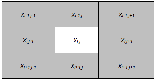
This neighborhood or interaction template can be chosen in several ways, although we will opt in our simulation for the one known as Moore's neighborhood (Fig. 2).
On the other hand, each cell
We will choose
A global configuration for cellular automaton
Finally, this dynamic of temporal evolution of the model is determined by the transition function p, which specifies how a cell changes state as a function of its previous state, and of its interaction with its vicinity of cells, according to equation:
where
Extensions of the definition given to include spatial or temporal homogeneity are feasible. If the AC is deterministic, the transition function leads to a single feasible state change, whereas if it is stochastic, the new state of a cell depends on some probability distribution.
4 Adeconocarcinoma Ductal in Situ Model with Cellular Automaton
To model the duct, a cellular automaton is used, with a tridimensional grid ζ with 20×20×200 nodes, which is built from the two-dimensional model proposed in [13] by adding an additional dimensional.
Each node can contain one cell. Although a human ductal cell has a genome composed of multiple genes with millions of DNA bases, we will limit ourselves to considering in the model only the four genes involved in the pathogenesis of the DICS, which are encoded by an integer of 32 bits [12]. The genetic load of a cell is then modelled by an ordered tuple of the form GC=(brca1, brca2, pten, tp53). The GC tuple is in turn coded by a single integer using the pairing function given by equation 5. Moore's vicinity extended to three dimensions and a null boundary condition are used to give the ends of the duct biological coherence:
In this way, GC is coded using the expression
The nodes of the grid are updated synchronously node by node of the duct and if they contain a cell of a given type, updating its genome according to its probability of mutation and its neighboring environment. Both variables define the transition function p. The selection and updating of the 8×l04 nodes of the the grid defines a generation, and the number of generations is varied depending on the length of the natural history of the tumor being simulated, increasing or decreasing the number of simulation generations. At this point, it is already evident that the computational load that the simulation imposes is very high, and that the parallelization of the model is obligatory to have computable simulations with reasonable execution times, or to simulate several ducts at the same time with different initial conditions or different natural histories.
The grid is initialized by a completely deterministic algorithm that creates a basal membrane and places a small number of progenitor cells inside it, which reproduce to form a double-layer duct that mimics the real biological formation for any human gland (Figure 3) with secretory function, although here we will apply it to the breast ducts.
Each cross section of the duct contains approximately 45-50 luminal cells. Originally, al the cells located in the duct have a healthy genome, represented by a chain of bits equal to zero. Mutations are modelled by putting one or more bits of a gene at a value of one. If the mode is to be executed considering an inherited genetic predisposition to contracting the disease, the HMG control flag is used, which allows this to be done, using a Monte-Carlo stochastic method.
The reticulum initialization algorithm, which allows obtaining a simulation of the duct compatible with the histological structure of a duct in the human breast, is illustrated as follows.1
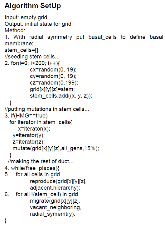
When the previous simulation is executed through our parallel implementation with the Java language, a grid is obtained (Figure 4) that coherently models the normal histological structure of a human duct (Figure 3), and all the cells generated in the grid remain inside, adopting the double layer structure illustrated in Figure 4 for the normal state of the duct.
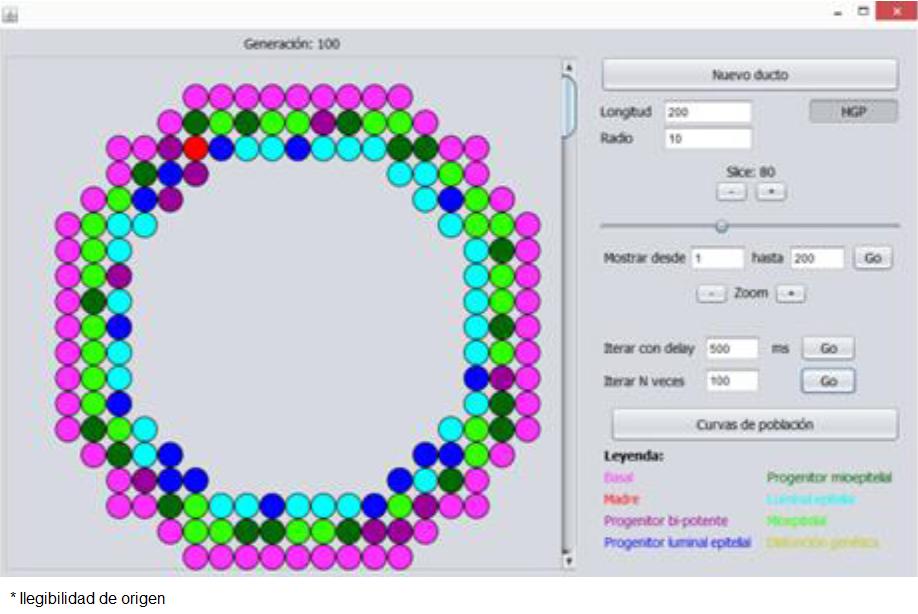
During the reproduction phase modeled on line number 5, all cells in the grid divide and occupy adjacent places, consistent with the parent hierarchy and provided there is room for it. The inherited genetic load can be mutated, according to the mutation rate set as a parameter of the mutate method, to which we have given a value [15] of 15%, which encompasses reasonably well the various real causes that can give rise to this type of mutations, and which include the environment, genetics and even the typology of the cell.
Since all genes are mutated through the method, including those that control both mitosis and programmed cell death, the cells in the duct resulting from the SetUp routine will eventually lead to neoplastic pathology. Once the grid is in its initial state, it is necessary to make it evolve over time, which is done by the Evolve algorithm.

In the above algorithm, methods BRCA1, BRCA2, PTEN and TP53 take the integer that encodes the genome of a cell from the grid and extract the 32-bit integer that encodes the gene that gives name to the method; the mutation method takes by argument a numerically encoded gene and returns the number of mutations it presents, as an integer between 0 and 32.
The adjacent_basal and adjacent_myopithelial methods allow us to know the typology of the cells that form the Moore neighborhood cube of the cell that take as argument while the adjacent_free method consults the neighborhood of free nodes for the node that takes as argument. For its part, there is also available a set of four methods that allow to know the type of cell that there is in a node of the grid. The normal_reproduction subroutine allows parents to reproduce themselves correctly, at points in their local cubic vicinity, and preserving the double-layer structure of the duct.
The cancerous_reproduction subroutine allows cells to reproduce indiscriminately at points in their local cubic vicinity, but does not respect the double-layer structure of the duct, and ends up forming an intraductal carcinoma in situ. Note that for a parent to be able to reproduce in this way, it is necessary that the total sum of mutations in its four genes be greater than half the positions that the four genes encode. Moreover, a simulation is carried out by determining a number of time steps, in each of which the Evolve algorithm described is executed. When a critical number of mutations is reached, the cells begin to proliferate uncontrollably, filling up the light in the duct and forming the carcinoma in situ.
Figure 5 illustrates this for several of a two hundred layer formed duct, where neoplastic transformation has taken place and malignant cells have begun to fill the duct light, without infiltrating the basement membrane.

As for the biological fidelity of the model used, we compared the simulation with a real specimen, using as a variable the number of neoplastic cells in the duct as a function of time (represented as the number of generations in the scope of the model).
In the real case, the genetic predisposition had been verified by means of immunohistochemistry methods, while in our case the corresponding flag of the simulation was activated. Figure 7 shows the comparison and, for both cases, the classic gompertzian behavior [6] is appreciated, which describes the tumoral dynamics both in vivo and in vitro, which tends to occupy the entire available tissue domain with a quasi-exponential acceleration from a certain point in time of evolution.
We see that in silico simulation is compatible with biological reality as well as the histological relaity, with an acceptable degree of fidelity to the global dynamics of neoplastic growth in situ.
5 Implementation
The previous model was implemented using the Java programming language, and parallelizing the sequential version obtained initially.
The parallelization uses the principles of symmetric multiprocessing with parallelism of data, dividing the reticule in its longitudinal ntroduce in cubic sections that were processed by different threads on a core dedicated to each one of them [17].
The tasks were supported by implementing the Runnable interface and processed through a ThreadPoolExecutor class object. In order to reduce containment to a minimum, two different ducts were used for reading and writing data. However, it was necessary to introduce two synchronization conditions:
a) barrier condition, in order to resynchronize all tasks when Evolve has been executed in time t and will be executed in time t+1.
b) collection of reentrant locks, which protect the contact zones between the different cubic sections into which the duct is divided, formed by two layers of each section, with the aim that two different strands cannot modify at the same time the same grid node and which certainly induce a relative degree of containment which, on the other hand, with the design of the data structure presented, is unavoidable.
It was also necessary to introduce a security condition to ensure that the simulation was coherent, consisting of forcing a thread that intends to write in the bi-layer section of the neighboring subretticle to consult the state of the node in which it intends to write [14], after having achieved the acquisition of the lock, since the thread responsible for that neighboring subretticle could have occupied that node in its own writing time. The execution tests were developed on four different nodes of the processor cluster of our university.
Each node has two Intel® processors Xeon™ E5 to 2.6 GHZ, which yield 20.8 GFLOPS together, with a common 128 GB memory bank, and without hyperthreading. The entry node operates the HP Cluster Management Utility on Red Hat Enterprise Linux for HPC. The version of the Java development kit used was Oracle 1.8.0.151-1.b12.e17_4. The statistical treatment of the data was carried out with R.
6 Measurements and Disccusion
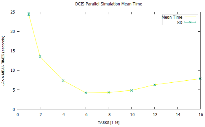
Figures 7 and 8 illustrate the mean times and speedups obtained from the simulation data in the four nodes of the cluster. Each point shows the mean time and speedup for a given number of tasks, also including the standard deviation (SD).

It can be seen that both the time curve and the speedup curve reach their relative extremes around the eight parallel tasks and that from here on, they begin to worsen if we increase the number of parallel tasks more. In other words, the optimum average time is 4.18 seconds for a maximum speedup of 5.85, over a theoretical maximum of 16, which is the number of cores available in each node, and starting from a sequential time of 24.45 seconds.
A priori one might think that a parallelization of the model that hardly accelerates half of the possible theoretical range is a parallelization that could be improved. Notwithstanding the above, it is necessary to qualify the why of these results, based on the following items:
a) It should be remembered that the contact zones between subgrids controlled by different strands are protected by a mutual exclusion block, which introduces latencies of waiting interthreads that are not dispensable because they guarantee the coherence of the state of the This directly induces a runtime overload that is proportional to the number of parallel strands (and contact zones) you have. This had been characterized by us in a previous paper [14] and independently by other authors for a problem of similar nature in [10].
b) Although the introduction of reticles of different readings and writing allow the tasks to be processed exclusively and completely parallel with the other strands of the nodes that are not in the contact zones of the reticule, the same does not happen with the nodes that are. Here, the thread that wants to write in a node located in the contact zone, once it has the permission to do so, cannot only use the neighborhood data that it had when it did its reading, but it must also consult the writing grid to verify that a modification occupying space is feasible, because perhaps another thread I occupied is space as a result of a mitosis. This also induces execution overloads.
c) Let us also remember that each node of the reticule encodes by means of a single positive integer number a lot of information (type of cell that occupies the node, and genes BRCA1, BRCA, PTEN and TP53. This means that the reading of the necessary information about the vicinity of a cell (adjacent_basal and adjacent_myoepithelial methods), the query of whether or not a cell is of the stem type or the induction of a mutation in a cell to name but a few, need to carry out the phases of decoding (and if necessary coding) numerical, all of which also adds an important processing load.
It could be thought that the representation of the state and genome of a cell by means of a gridCell class could improve this last aspect, although the measures we have taken for this case, developing an alterantive implementation with it, discard it in a radical way. The space occupied in the heap of the Java Virtual Machine by the nodes modeled as classes, and the need to navigate their respective references to reach them, increases global processing times and decreases speedups.
In short, the three previous items justify why the speedups obtained, the second one being especially relevant, and being also coherent with models that develop similar simulation dynamics in two dimensions, such as the results published in [10,14].
7 Conclussions and Future Work
The work presented proposes a general procedure for parallel simulation of adenocarcinomas in situ, using the cellular automata model. As it has been presented, the simple change of the transition function of the cellular automaton in the two proposed algorithms and of the genetic load model allows it to be adapted to different types of glandular neoplasms before they adopt an infiltrating character. From the proposed algorithms, a parallel implementation has been made using Java language with symmetric multiprocessing by parallelism of data for the study of a case: ductal adenocarcinoma of breast in situ.
The parallel simulation in the cluster of processors of our University has allowed a reduction of the processing times (Figure 7) achieving a maximum speedup factor of 5.85 (Figure 8); it has also allowed us to identify an important limitation to the scalability of the proposed method, derived from the need to have under control of mutual exclusion the nodes of the simulation grid located in contact zones of the data spaces of different threads, which we had already identified in a previous work \cite{sal} for a simulation in two dimensions.
This limitation is specific to the nature of the problem and therefore cannot be overlooked. The fidelity of the proposed model has also been contrasted with biological reality by means of the construction of the curves illustrated in Figure 6, which show that the simulation achieves, with more than acceptable fidelity, the usual sharing in this type of neoplasms.

Our future lines of work on the proposed model will be oriented towards:

