


 text new page (beta)
 English (pdf)
 Article in xml format
 Article references
 Send this article by e-mail
 Cited by SciELO
  Similars in
SciELO
Similars in
SciELO 
 Permalink
1 Introduction
The μ-calculus is an extension of the propositional modal logic with least and greatest fixed-points. This logic subsumes many temporal, modal and description logics (DLs), such as the Propositional Dynamic Logic (PDL) and the Computation Tree Logic (CTL) [10,9]. Due to its expressive power and nice computational properties, the μ-calculus has been extensively used in many areas of computer science, such as program verification, concurrent systems and knowledge representation. In this last domain, the μ-calculus has been particularly useful in the identification of expressive and computationally well-behaved DLs [10], which are used as the web ontology language OWL, now a standard technology for the W3C. Another standard for the W3C is the XPath query language for XML.
XPath also takes an important role in many XML technologies, such as XProc, XSLT and XQuery. Due to its capability to express recursive and multi-directional navigation, the μ-calculus has also been successfully used as a framework for the evaluation and reasoning of XPath queries [5,4,12]. However, extending (Presburger) arithmetical constraints for XPath queries leads to undecidablity [36]. In the current paper, we identify a decidable extension, vía a logic characterization, of XPath queries with Presburger arithmetical constraints on children paths.
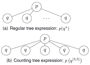
The μ-calculus is as expressive as the monadic second order logic (MSO) [12], it has thus been successfully used in the XML setting in the description of schema languages [4], which can be seen as the tree version of regular expressions. Analogously as regular expressions are interpreted as sets of strings, XML schemas (regular tree expressions) are interpreted as sets of unranked trees (XML documents). For example, expression p(q*) represents the sets of trees rooted at p with either none, one or more children subtrees matching q. See Figure 1(a) for an interpretation of p(q*). Counting operators impose occurrence bounds on children [28]. For instance, p(q [3,5])) denotes the trees rooted at p, with at least 3 but no more than 5 children matching q. In Figure 1(b), it is depicted an interpretation of p(q [3,5])). In the present work, we proposea new EXPTIME decision algorithm for regular tree languages with counting operators. Furthermore, we also identify a new extension of regular tree languages with the interleaving operator [27]. This extension has also an EXPTIME upper bound. This operator is used to denote the trees resulting from the permutation of siblings, and it has also applications in algebraic approaches of concurrent computation models. Also, in XML schema languages there are interleaving operators, such as in RelaxNG.
1.1 Related Work
The extension of the μ-calculus with nominals, inverse programs and graded modalities is known as the fully enriched μ-calculus [10]. Nominals are intuitively interpreted as singleton sets, inverse programs are used to express past properties (backward navigation along accesability relations), and graded modalities express numerical constraints on the number immediate successor nodes [10]. However, satisfiability/validity of the fully enriched μ-calculus was proven by Bonattiand Peron to be undecidable [11]. Nevertheless, Barcenas et al. [4] recently showed that the fully enriched μ-calculus is decidable in single exponential time when its interpretations are restricted to finite trees. Graded modalities in the context of trees are used to constrain the number of children nodes with respect to natural numbers. In this work, we introduce a generalization of graded modalities.
This generalization considers numerical bounds on children with respect to Presburger arithmetical expressions, as for instance ϕ>ψ, which restricts the number of children where ϕ holds to be strictly greater than the number of children where ψ is true. Other works have previously considered Presburger constraints on tree logics. MSO with Presburger constraints was shown to be undecidable by Seidl et al. [31]. Demri and Lugiez proved a PSPACE-complete bound on the propositional modal logic with Presburger constraints [16]. A tree logic with a fixed-point and Presburger constraints was shown to be decidable in EXPTIME by Seidl et al. [33,32]. In the current work, we push decidability further by allowing nominals and inverse programs in addition to Presburger constraints.
Regarding expressiveness, in [17] is proposed an extension of MSO with
counting on unranked trees, together with the corresponding weighted automata.
Other forms of counting considering more extensive tree regions, such as
ancestors or descendants, have been studied in [37,2,8,39,5,34,1,24], however in contrast with the current
work, these works consider node occurrence constraints with respect to natural
numbers only. An extension of first order logic with two variables
FO2 with counting quantifiers interpreted over two forests of
ranked trees was recently proposed in [13,14]. The counting quantifiers consist of
existential
As in this article, Fischer-Ladner satisfiability algorithms for counting extensions of the μ-calculus for trees are introduced in [4,5].
In these works, it was also showed that these counting constraints with respect to numbers only, although exponentially more succinct, does not introduce extra-expressive power. This allowed to use the traditional Fixed-Point Theorem for the μ-calculus to prove the algorithm correctness. Contrastingly, in the current work we propose a counting extension of the μ-calculus with full Presburger arithmetic, which clearly implies more expressive power. In order to prove the algorithm correctness, we prove a generalization of the Fixed-Point Theorem for the Presburger extension of the μ-calculus for trees, which is also technical result of independent interest.
Complexity and succinctness of regular tree (string) languages extended with counting and interleaving operators have been extensively studied in [28,27,19,4,15]. In [19], Gelade shows that the interleaving operator is exponentially more succinct, even when it is directly encoded by tree automata. It is also shown that hardcoding counting operators produces doubly exponential larger expressions. Meyer and Stockmeyer showed in [28] that the equivalence of regular expressions with counting operators is EXPSPACE-complete. EXPSPACE completeness of the equivalence of regular expressions with interleaving was proven in [27].
In [4], it is described and extension of regular trees expressions with counting and interleaving, where emptiness, containment and equivalence are decidable in EXPTIME. In the current work, we identify further extensions of interleaving occurring in recursive and disjunctive fragments. Emptiness, containment and equivalence are also proved to be EXPTIME.
Regarding counting, operators introduced in [4], although impose occurrence bounds on children, do not restrict the consecutive occurrence of children. This contrasts with traditional semantics of counting in regular languages [28,19]. In the current work, by means of Presburger constraints, we identify an extension of regular tree expressions with traditional counting operators decidable in EXPTIME. In [15], it is introduced a polynomial algorithm for the containment of regular trees with both counting and interleaving.
The algorithm assumes two main restrictions on tree expressions: propositions occur only once, and counting can be applied to propositions only. The EXPTIME algorithm proposed in the current work overcomes these two limitations.
Counting operators on regular paths (XPath) have been studied before in [36,4,5]. ten Cate and Marx [36] showed that Presburger constraints on full regular paths lead to an undecidable formalism.
In [4], it was shown that when restricting only children with respect to a natural number (encoded in binary), reasoning (emptiness, containment and equivalence) is in EXPTIME. This result was extended to operators capable of constraining (w.r.t. a binary number) any regular path, including ancestors, descendants, compositions, etc. [5]. In this paper, we show that full Presbuger arithmetic becomes decidable on children paths. Furthermore, we set new optimal EXPTIME bounds for containment and equivalence on full (multi-directional) regular paths with Presburger constraints on children.
1.2 Outline
We introduce a modal logic for trees with fixed-points, inverse programs, and Presburger constraints in Section 2.
In Section 3, an EXPTIME satisfiability algorithm is described and proved correct. Also, it is shown that the computational cost of the algorithm is single exponential time with respect to the size of the input formula, even if the Presburger constraints are encoded in binary form.
In Section 4, we introduce extensions of regular tree languages with counting and interleaving operators.
In Section 5, regular path queries extended with Presburger constraints on children are introduced. Both extensions of regular trees and paths are shown to be succinctly captured in terms of logic formulas. This implies the satisfiability algorithm can be used as an optimal reasoning framework for regular trees and paths with counting and interleaving.
A summary together with a discussion of further research perspectives are reported in Section 6.
2 Tree Logic with Recursion, Inverse, and Presburger Constraints
In this section, we introduce an expressive modal logic for finite unranked tree models. The tree logic (TL) is equipped with operators for recursion (μ), inverse programs (I), and Presburger constraints (C). This logic can be seen as the fully enriched μ-calculus [10], extended with Presburger constraints, interpreted over tree structures.
2.1 Syntax and Semantics
We first consider a set of propositions P, a finite set of modalities M={↓,→,↑,←}, and a set of variables X.
Definition 1 (μTLIC syntax). The set of μTLIC formulas is defined by the following grammar:
where
In order to provide a formal semantics, we need some preliminaries. A tree
structure
—
— the set of nodes
—
—
In the setting of XML documents (unranked trees), node labels are defined by a function instead of a relation, that is, exactly one proposition holds at each node. The satisfiability algorithm described in Section 3 can easily be adapted for this restriction (see Definition 6).
Given a tree structure, a valuation V of variables is defined as
a function from the set variables X to a set of nodes
Definition 2 (μTLIC semantics). Given a tree
structure
We say a tree
The satisfiability problem for μTLIC consists in deciding whether or not a given formula is satisfiable.
We now give an intuition about the interpretation of formulas: propositions
p are node labels; negation and disjunction are interpreted
as the complement and the union of sets, respectively; modal formulas
We also use the following traditional notation:
Note that
Examples
Consider for instance the following formula ψ:
where (r ≤ 2q) stands for 1r + (-2)q ≤ 0. ψ is true in nodes labeled by p, such that the number of its q children is at least twice the number of its r children. This is a common example that goes beyond the expressive power of (graded) μ-calculus and regular languages [16].
In Figure 2, there is a graphical representation of a model for ψ:

It is also possible to express recursive navigation, for example, consider the following formula ϕ:
ϕ is true in nodes with at least one descendant where ψ is true, that is, ϕ recursively navigates along children until it finds a ψ node.
Backward navigation may also be expressible with the help of inverse programs (converse modalities). For instance, consider the following formula φ:
φ holds in nodes with an ancestor where ψ is true, that is, φ recursively navigates along parents until it finds a ψ node. Furthermore, in contrast with other approaches without converse modalities [16,32], this new feature allows to count also on sibling nodes. For instance:
holds in nodes with more than 10 siblings named p.
2.2 Other Forms of Counting
We now show how several notions of counting (nominals, graded modalities and global counting) can also be expressed in terms of μTLIC formulas.
Hybrid Logics
The interpretation of nominals is a singleton, that is, nominals are formulas which are true in exactly one node in the entire model [9]. Now, it is easy to see that μTLIC can navigate recursively thanks to the fixed-points, and in all directions thanks to inverse programs.
Hence, μTLIC can then express for a formula to be true in one node while being false in all other nodes of the model. Nominals are then defined as follows:
where formulas Siblings(ϕ), Ancestors(ϕ), and Descendants(ϕ) are true, if and only if, ϕ is true in all siblings, ancestors, and descendants, respectively. More precisely:
Graded Logics
In modal logics, graded modalities are specialized operators for expressing
numerical bounds on the occurrence of a sole formula in adjacent nodes. In the
context of tree models, the numerical bounds are on children nodes
[4].
For instance, formula
where k is a positive integer number encoded in binary.
Global Counting
Global numerical constraints, as its name suggest, are operators used to impose constraints on the occurrence of a sole formula with respect to a constant in the entire model [37,2,39,5].
That is, a formula ϕ>G k holds in the entire model, if and only if, ϕ is satisfied by at least k + 1 nodes. More precisely, the interpretation of global counting formulas with respect to a tree 𝒯 and a valuation V is the following:
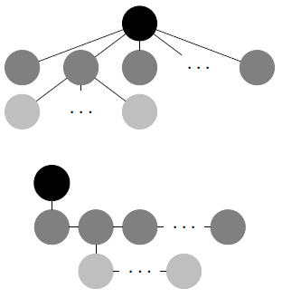
Note that the intended interpretation of ϕ≤G k is the same as for formula ¬(ϕ>G k). In [5], it was shown that regular path queries (XPath) with numerical constraints on any path, for instance ancestors or descendants, can be succinctly expressed by global counting formulas. It was also shown in [5] that global numerical constraints does not provided extra expressive power by means of a reduction to the two-way μ-calculus (without counting). More precisely, for any binary tree T (for technical convenience, binary trees are used instead of n-ary trees, there is a well known bijection between them, see Figure 3 on page 7) and valuation V, we have the following:
where r stands for the root node
μTLIC can therefore also express global numerical constraints. However, it is not hard to see that hardcoding of global numerical constraints comes at an exponential cost [5].
3 Satisfiability
In the current section, we describe a satisfiability algorithm for the logic μTLIC. That is, given an input μTLIC formula, the algorithm decides whether or not there is a tree model satisfying the formula. The algorithm inspired from the well-known Fischer-Ladner approach [18] and the binary encoding of counting constraints introduced in [5,4]. Candidate trees are enumerated starting from the single nodes (leaves). Then, parents are iteratively added until a satisfying tree is found. The stop condition for this iterative process is given by the number of available nodes, which are defined as sets of subformulas (of the input formula). These subformulas represents the information required to build the trees: node names, tree topology, Presburger constraints. One notable distinction of our algorithm is that Presburger constraints are encoded in binary form.
Before describing the algorithm, we describe the notion of trees. Then we show that the algorithm is correct and in EXPTIME.
3.1 Fischer-Ladner-Presburger Trees
We first give a detailed description of the syntactic version of tree models constructed by the satisfiability algorithm.
Some preliminaries are now introduced. There is well-known bijection between
binary and n-ary trees [22]. One adjacency is interpreted as
the first child relation and the other adjacency is for the right sibling
relation. In Figure 3 is depicted an
example of the bijection. Hence, without loss of generality, from now on, we
consider binary unranked trees only. At the logic level, formulas are
interpreted as expected:
For the satisfiability algorithm we consider formulas in negation normal form only.
The negation normal form (NNF) of μTLIC formulas is defined by the usual De Morgan rules and the following ones:
Hence, negation symbol ¬ in formulas in NNF occurs only in front of propositions
and formulas of the form
From now on, we often write γ#b to denote any of the following formulas: γ > b or γ ≤ b.
We now consider a binary encoding of natural numbers. Given a finite set of
propositions, the binary encoding of a natural number is the Boolean combination
of propositions satisfying the binary representation of the given number. For
example, number 0 is written
Definition 3 (Counters). Given a formula ϕ and a number b > 0, a counter of ϕ set to k is defined by:
where
Consider for instance the counter of formula ϕ set to 7:
We write (C(ϕ)=b) ∈
S, when each ϕi ∈
S where
A formula ϕ induces a set of counters corresponding to its counting subformulas. The bound on the number of propositions used by counters is given by K(ϕ), and it is proved in Theorem 5.
Nodes in Fischer-Ladner-Presburger trees are defined as sets of subformulas. These subformulas are extracted with the help of the Fischer-Ladner-Presburger Closure. Before defining the Closure, we define the following set of subformulas of a counting expression:
We often write ϕγ to denote ϕ ∈ S(γ).
Now, consider the following binary relation RFLP on
the set of μTLIC formulas, for
Definition 4 (Fischer-Ladner-Presburger Closure). Given a formula
ϕ, the Fischer-Ladner-Presburger Closure of
ϕ is defined as
Example 1. Consider the following formula:
This formula holds in p nodes with at least one more q child with respect to r children. In Figure 4, there is graphical representation of a ϕ-tree (Definition 7) for formula ϕ. In the definition of ϕ-trees, we use the notion of Fischer-Ladner-Presburger closure, which in the case of ϕ is defined as follows for j = 0,1,2:
We are now ready to define the lean set for nodes in Fischer-Ladner-Presburger trees. The lean set contains the propositions, modal subformulas, counters and counting subformulas of the formula in question (for the satisfiability algorithm). Intuitively, propositions will serve to label nodes, modal subformulas contain the topological information of the trees, and counters are used to verify the satisfaction of counting constraints.
Definition 5 (Lean). Given a formula ϕ, its lean set is defined as follows:
provided that p’ does not occur in ϕ , and m =, ↓, →, ↑, ←.
Example 2. Consider again the formula
Where
Recall that qj and rj are the corresponding propositions (associated to q and r) required to define the corresponding binary encoding of numbers.
Definition 6. The set of ϕ-nodes is defined as follows:
Intuitively, a ϕ-node
— at least (exactly1) one proposition (different from the counter propositions) occurs in
— if a modal subformula
— both
When it is clear from the context, ϕ-nodes are called simply nodes.
We are finally ready to define the Fischer-Lander-Presburger ϕ-trees.
Definition 7. A ϕ-tree is defined:
— either as empty ∅, or
— as a triple
The root of
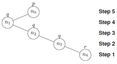
Example 3. Consider again the following formula
ϕ-nodes ni (i = 0,...,4) are defined from the lean of ϕ (Example 2). In Figure 4 is depicted a graphical representation of T. Notice that counters in the root n0 are set to zero 0, that is, no proposition corresponding to counters occurs. This is because counters are intended to count siblings only. For instance, counters in n1 are set to 3 and 1 for q and r, respectively, because there are three q's and one r in n1 and its siblings. Counting formulas occur positively only at the root n0, because they are intended to be true when the counters in the children of n0 satisfy the Presburger constraints. Since ni(i > 0) does not have children, then counting formulas occur negatively (recall the negation normal form of the input formula is also in the lean) in these nodes. Finally, notice that modal subformulas define the topology of the tree.
3.2 The Algorithm
We now define a satisfiability algorithm for the logic μTLIC following the Fischer-Ladner method [5,4,16,18]. Given an input formula, the algorithm decides whether or not the formula is satisfiable. The algorithm builds ϕ-trees in a bottom-up manner. Starting from the leaves, parents are iteratively added until a satisfying tree, with respect to ϕ, is found.
Algorithm 1 describes the bottom-up construction of ϕ-trees.

The set Init(ϕ) gathers the leaves. The
satisfiability of formulas with respect to ϕ-trees is tested
with the entailment relation
Example 4. Consider the formula
We now give a detailed description of the algorithm components.
Definition 8 (Entailment). The entailment relation is defined as follows:
If there is a node n in a tree T, such that
n entails
Leaves are ϕ-nodes without downward adjacencies, that is,
formulas with the form
Definition 9 (Init). Given a formula ϕ, its initial set Init(ϕ) is defined as follows:
Notice that, from definition of ϕ-nodes, if formulas of the
forms
Example 5. Consider again the formula ϕ of
Example 3. It is then easy to see that n4 is a leaf.
n4 does not contain downward modal formulas
The Update function consistently adds parents to previously
built trees. Consistency is defined with respect to two different notions. One
notion is with respect to modal formulas. For example, a modal formula
Definition 10 (Modal Consistency). Given a ϕ-node
Example 6. Consider ϕ in Figure 4. In step 2, it is easy to see that
n3 is modally consistent with
n4: formula
Another consistency notion is defined in terms of counters. Since the first child is the upper one in a tree, it must contain all the information regarding counters, i.e., each time a previous sibling is added by the algorithm, counters must be updated. Counter consistency must also consider that counting formulas occurs in the parents, if and only if, the counters of its first child are consistent with constraints in counting subformulas.
Definition 11 (Counter Consistency). Given a ϕ-node
Example 7. Consider the formula ϕ of Example 3 and Figure 4. In steps 2, 3 and 4, since previous siblings are added, counters for q are incremented in n3, n2 and n1, respectively. In step 5, the counting formulas q-r>1 and r>0 are present in the root n0, due to the fact that counters, in the first child, satisfy the Presburger constraints.
Update function gathers the notions of counter and modal consistency.
Definition 12 (Update). Given a set of ϕ-trees X and set of ϕ-nodes Y, the update function is defined as follow for i = 1,2:
We finally define the function root(X), which takes as input a set of ϕ-trees and returns a set with the roots of the ϕ -trees.
3.3 Correctness
We now show that Algorithm 1 is correct, and then we describe its complexity. Correctness is shown by proving that the algorithm is sound and complete. For these proofs, we first need a fixed point theorem. Proving substitution is monotone is the first step.
Lemma 1.
Given a μTLIC formula ϕ, a tree structure
Proof. We proceed by induction on the structure of
ϕ. Base cases are trivial and most inductive cases are
straightforward by inductive hypothesis. Recall that since we are considering
only formulas in negated normal form, negation symbols ¬ occur in front of
propositions and formulas
The case of the Presburger formula γ > b is more interesting.
We prove this case by a second induction on the structure of γ. We distinguish
three base cases, the first one is
Consider now the case for
We now prove the fixed point Theorem.
Theorem 1.
Given a μTLIC formula ϕ, a tree structure
Proof. Since
A straightforward observation from the fixed point Theorem 1 is that a fixed
point μx.ϕ is equivalent to its unfolding
Theorem 2 (Soundness). If the satisfiability algorithm returns that ϕ is satisfiable, then there is tree model satisfying ϕ.
Proof. Assume T is the ϕ-tree
that entails ϕ. Then we construct a tree model
— the nodes of
— for each triple (n, T1, T2) in T,
— if p ∈ n, then p ∈ L(n).
We now show by induction on the structure of the input formula ϕ
that
Base cases are immediate, that is, when the input formula is either a
proposition, a negated proposition or formulas with the form
Negations and disjunctions are also immediate by induction. Modal formulas
Also in T, we know that n is the first child of
a node n0 where
Completeness proof is divided in two main steps: first we show that there is a lean labeled version of the satisfying model; and then we show that the algorithm can actually build the lean labeled version of the tree model.
Theorem 3.
If there is a tree structure
Proof. Assume
It is now shown by induction on the derivation of
Before proving that the algorithm builds T, we need to show that there are enough ϕ-nodes to construct T. Recall ϕ-nodes are lean subsets, and the lean is composed by propositions, modal and counting formulas occurring in the input formula, plus counters. Since counters count children nodes, we then need a bound on the number of children. For this purpose, we use a bound of an integer programming problem.
Theorem 4.
[30]
Let A be a m × n integer matrix and b a m-vector, both with entries in
ℤ. Then if Ax = b has a solution
Theorem 5. If a formula ϕ is satisfiable, then there is a ϕ-tree entailing ϕ where each node has at most an exponential number of children with respect to the size of ϕ.
Proof. Since ϕ is satisfiable, there is a
ϕ-tree T entailing ϕ by
Theorem 3. Recall each node in T is a subset of
lean(ϕ), thus composed by propositions, modal formulas
We are now ready to show that the algorithm builds the lean labeled version
T of the satisfying model
Theorem 6 (Completeness). If there is a tree model
Proof. The proof proceeds by induction on the height of
Theorem 7 (Complexity). μTLIC satisfiability is EXPTIME-complete.
Proof. We first show that the lean set of the input formula ϕ has linear size with respect to the size of ϕ. This is easily proven by induction on the structure ϕ and by Theorem 5: an exponential number of children can be distinguished by a linear amount of counting propositions (recall counters are encoded in binary). We then proceed to show that the algorithm takes exponential time with respect to the size of the lean. Since ϕ-nodes are defined as subsets of the lean, it is then clear that the number of ϕ-nodes is single exponential with respect to lean size, then there is at most an exponential number of steps in the loop of the algorithm.
It remains to prove that each step, including the ones inside the loop, takes at
most exponential time: computing Init(ϕ)
implies the traversal of
4 Extended Regular Tree Languages
In this section, we introduce several extensions of regular tree languages, which encompass most XML schema languages used in practice, such as DTDs, XML Schema and RelaxNG [29,22]. First we consider the extension with the interleaving operator [27]. Then the extension with counting operators [28]. We show that these extension can be linearly characterized by μTLIC. In Section 5, we also show that regular path queries (XPath) [36] with Presbuger constraints on children path can also be linearly expressed by μTLIC. As a consequence, μTLIC can be used as a framework for standard XML reasoning problems involving schemas and queries with counting and interleaving operators. In Section 3, we describe an EXPTIME satisfiability algorithm, which together with results described in this Section, imply new optimal (EXPTIME) bounds on emptiness, inclusion and equivalence of XPath queries (with counting) and XML schemas (with counting and interleaving).
4.1 Regular Tree Languages
We define the syntax of regular trees similarly as in [20,22].
Definition 13 (Syntax of regular trees). We define the set of regular tree expressions by the following grammar:
We write p instead of
Following [22], we now give a precise semantics of
regular tree expressions, but first, we define the following notation. Consider
a tree structure
Definition 14 (Semantics of regular trees). Given a valuation V (from variables to sets of trees), regular tree expressions are interpreted as follows:
where lfp
Note that there is always a least fixed poir due to the Knaster-TarskiTheorem [35] on fixe< points (substitution is monotone with respect to th subset ordering).
Intuitively, regular tree expressions are interpreted as sets of unranked trees:
We now show that regular tree expressions can linearly be translated in terms of
the μ-calculus, as already shown in [4,5]. This implies that
traditional reasoning problems, such as emptiness, containment (inclusion) and
equivalence, can be efficiently expressed in terms of the satisfiability of
μ-calculus formulas. Before defining a translation function
from regular tree expressions to logic formulas, we define
Definition 15. We define the following translation function from regular tree expressions to μ-calculus formulas:
where
—
—
—
—
We say an expression e is nullable when it is a variable bounded
to an expression that can be interpreted as the empty tree, as for instance
Now, consider as an example the expression
Theorem 8 (Reasoning on regular trees [4,5]). Given any
two regular tree expressions e1 and e2, we have that
for any tree
4.2 Interleaving
The interleaving operator, sometimes called shuffle operator, is a common extension of regular languages [27]. In particular, there is an interleaving operator in XML Schema and RelaxNG. Intuitively, the interleave of two regular tree expressions matches the concatenation of trees corresponding to the expressions regardless their order. This operator does not introduce more expressive power to regular languages, however, it is double-exponentially more succinct [19]. For instance, the interleaving of expressions pq and rs can be described as follows:
Definition 16 (Interleaving). The interleaving operator in regular tree expressions is inductively defined as follows:
Counting formulas in μTLIC can be used to represent the interleaving of regular tree expressions. For this purpose, we restrict the expressions that can be interleaved. This restriction is defined by the following grammar:
where e is a regular tree expression without restrictions
(Definition 13), and disjunctions have constant size, that is, for expressions
For instance, expressions of the form p&q* are disallowed, notice however that recursion can occur at another level of interleaving, for instance, p&r[q*]. Now for an example of constant size disjunctions, (ppp+ qq)&rrr is not allowed, because |ppp|* ≠ |qq|*. Instead, equally sized disjunction can occur at the same level of interleaving, for example (ppp+qqq)&rrr. Notice this restriction applies at top level only, hence expressions as the following are perfectly allowed s[ppp+qq]rrr.
We then define the translation of interleaving as follows.
Definition 17 (Translation of interleaving). Given two regular tree
expressions
The translation F of unrestricted regular tree expressions is given in Definition 15, and chsize is defined as follows:
Intuitively, chsize computes the number of children to be interleaved.
As an example consider the expression p[qr&st]. This can be expressed in terms of μTLIC as follows:
Note that concatenation order is preserved, that is, q goes always first than r, and s goes first than t. However, none other order restriction is imposed, hence, p, q, r, s may occur interleaved, as long as we know there are only 4 children.
From Theorem 8 and Definition 17, it is now easy to see we can efficiently reason on regular expressions with interleaving in terms of the satisfiability of μTLIC formulas.
Theorem 9 (Reasoning on regular trees with interleaving).
Given any two regular tree expressions e1 and
e2 with interleaving, we have that for any tree
—
—
—
Proof. For the first item, the proof goes by induction on the
structure of e1. All cases are identical as in
Theorem 8. We only show here the case of interleaving, that is, when
e1 has the form
Now, it is proved by induction that
The argument in this case also goes as the correspoding case of Theorem 8. Consider now this case:
Which is is immediate since
Now,
The second item is analogous. And the third one is straightforward by noticing F does not introduce duplications.
4.3 Counting
Counting operators in regular languages restrict the occurrences of expressions
with respect to natural numbers. For instance,
As one may easily notice, this counting operators do not provided more expressive power, however, they are exponentially more succinct [19], that is, expressing p[a,b], where a and b are natural numbers encoded in binary, results in an exponentially larger regular expression (without counting constructors).
One may think that counting restrictions in regular languages may be easily expressed by counting formulas in μTLIC, however, recall that counting formulas do not impose any occurrence order, whereas counting restrictions in regular languages do, expressions must be consecutively concatenated. In contrast with counting regular expressions in [4,5], where there is no order preservation, here we show that counting Presburger formulas may impose order restrictions on counting regular expressions, as in [28,19]. Furthermore, in the current work, we consider a more general form of the counting than [28,19], because counting expressions may no exhibit an upper bound.
Definition 18 (Counting regular tree expressions). Counting regular tree expressions are defined as follows:
where e’ is a regular expression without recursion at top level,
that is,
Intuitively,
This can be see as a generalization of the Kleene star, which can be expressed by
Definition 19 (Translation of counting). We translate the counting operator as follows:
where e’ is a regular expression without recursion at top level.
Consider as an example the following expression:
This formula means that q nodes have at least 2 p children, but no more than 5.
From Theorem 8 and Definition 19 we clearly can imply reasoning on regular expressions with counting and interleaving in terms of the satisfiability of μTLIC formulas. One may have noticed that the translation of counting regular tree expressions is not linear when considering the resulting counting formula as syntactic sugar. We then consider μTLIC extended in the obvious way with the additional counting operators. In Section 3, we present a satisfiability algorithm for μTLIC that can be easily extended with the syntactic sugar operator for counting.
Theorem 10 (Reasoning on regular trees with interleaving and counting). Given any two regular tree expressions e1 and e2 with interleaving and counting operators, we have that for any tree 𝒯 and valuations V and V’ the following holds:
—
—
—
Proof. For the first item, the proof goes by induction on the
structure of e1. All cases are identical as in
Theorem 8. The case of interleaving was shown in Theorem 9. Here, we only show
the case of counting:
This was already showed in the proof of Theorem 9. Then, it follows that
The second item is analogous. And the third one is straightforward by noticing F does not introduce duplications.
5 Regular Counting Paths
XPath is a query language for semi-structured data (XML), its navigation core is known as regular paths, and it corresponds to the First Order Logic with two variables FO2 [26]. We now introduce an extension of regular paths, considered in the specification of XPath [36], consisting of Presburger arithmetical constraints on children paths, that is, regular paths expressing children relations. We also give a new EXPTIME bound for reasoning on this counting extension of regular paths.
Definition 20 (Counting paths syntax). We inductively define regular paths expressions with Presburger constraints by the following grammar:
where p is a proposition and a and b are integers encoded in binary, b is non-negative.
In order to ensure decidability, path expressions occuring in the scope of a counting operator > are restricted to children, that is, they are expression of the forms: ↓,↓:p,↓[β] or ↓:p[β].
We now give a formal description of the interpretation of regular paths with Presburger constraints.
Definition 21 (Counting paths semantics). Given a tree structure
where
Intuitively, regular paths are interpreted over tree structures as pairs of nodes.
The left nodes, known as the context, represent from where the path is evaluated,
and the right nodes, denote the selection of the path. Axis relation ↓, as in
μTLIC, stands for the children relation, → for the following
sibling relation, ↑ for parents, ← for previous siblings,
So basic paths α : p denotes pair of nodes, such that the right node
of the pair is labeled by p and it is related with the left node of
the pair by α. So for instance,
where # stands for <, ≤, ≥, =. /ρ stands for the pair of nodes denoted by
p, such that the left node of the pairs is the root. Union,
intersection and difference of paths are expressed as
Regular paths can be linearly translated in terms of μ-calculus
[4].
Consider for instance the following expression:
Arithmetical constraints on children path can be expressed by μTLIC
counting expressions. For example,
As another example consider
When characterizing regular paths in terms of μTLIC formulas, we can denote the context from where paths are evaluated by some other formula. We usually denote this context formula by C.
Definition 22 (Translation of counting paths). We define the translation of regular paths with Presburger constraints, with respect to a context formula C, as follows:
where the translation of qualifiers F' is defined as follows.
where
From this translation, it is then clear that μTLIC can be used as a query reasoning framework for regular paths with Presburger constraints.
Theorem 11 (Counting paths reasoning). For any regular path
query with Presburger constraints ρ1 and ρ2, any formula
C, any tree structure
—
—
—
Proof. The proof of the first item goes by induction on the
structure of the input query. Base cases are immediate, as well as most inductive
ones. We will only consider then the case when the input query has the following
form:
Now, by induction, we know that for any tree
Since ap > b holds in nodes with more than b children, it is then easy to see that:
Other base cases for κ are analogous. Consider now the following input query
As in the base cases, by structural induction on paths, we know that
The second item is an immediate consequence of the first one.
Regarding the third item, since the translation does not introduce duplications (Definition 22), the proof goes straightforward by structural induction.
Corollary 1 (Query reasoning in the presence of schemas). Given
any two regular tree expressions e1 and e2 with
interleaving and counting operators, any regular paths with Presburger
constraints
— A query ρ1 is empty in the presence of a regular tree (schema) e1 , if and only if,
—a query ρ1 in the presence of a regular tree (schema) e1 is contained in a query ρ2 in the presence of a regular tree e2, if and only if,
—
6 Conclusions
We introduced a modal logic for trees with a fixed point, inverse programs, and Presburger constraints (μTLIC). This logic can been seen as the fully enriched μ-calculus for trees extended with Presburger constraints.
Regular tree languages (XML schemas) can be linearly captured by the logic. We introduced extensions of regular trees with interleaving and counting operators. These extensions can also be linearly characterized by μTLIC. Moreover, regular path queries (XPath) with Presburger constraints on children paths are also linearly translated in terms of μTLIC formulas.
Since the logic is closed under negation, it can be used as a XML reasoning framework for counting extensions of XPath and XML schemas. We showed that the logic is decidable in single exponential time, even if the Presbuger constraints are encoded in binary.
This result implies new EXPTIME bounds on XPath counting fragments and regular tree extensions with interleaving and counting.
In [6,3], decidable classes of ranked trees with counting and (dis)equality constraints are studied. As a further research perspective, we are interested in the relation of counting and equality constraints on unranked trees. We believe efficient decidability algorithms may be extracted from the modal logic approach.
In another setting, arithmetical constraints on trees have been also successfully used in the verification of balanced tree structures such as AVL or red-black trees [25,21].
We believe another field of application for the logic presented in the current work is in the verification of balanced tree structures. We also believe the logic can be used as an expressive framework in context-aware systems [7,23], where counting constraints play a key role when modeling location/distance variables.

