


 text new page (beta)
 English (pdf)
 Article in xml format
 Article references
 Send this article by e-mail
 Cited by SciELO
  Similars in
SciELO
Similars in
SciELO 
 Permalink
1 Introduction
Fractal analysis is a method to measure the complexity of shapes and structures. It has applications in many areas of science and engineering such as income distributions, money flow, sales data and daily temperature records, [1,2]. Electroencephalography signals [3] leakage current in high voltage insulators, [4,5] and tumors in mammographic images [6]. Around the world, the manufacturing industry of polymeric insulators has evolved rapidly over the past few years.
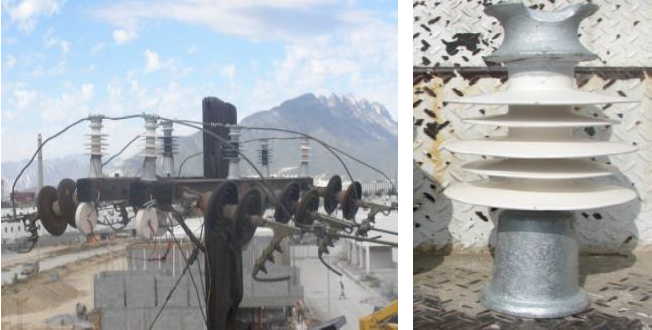
In several countries, research is mainly focused on developing resistant polymeric insulators to high levels of electric stress and pollution [7]. The use of polymeric insulators ranges from transmission lines, distribution lines and substations. Figure 1 shows polymeric insulators in a distribution line. Polymeric insulators have many advantages over their ceramic ones: lighter weight, high performance in contaminated environments, reduced maintenance and ease of installation [8].
Because there are a large number of brands and designs of polymeric insulators in the market, it is important to determine which the best insulator is with respect to others, in order to differentiate bad quality or bad designs. Currently several tracking and erosion aging tests are available for the assessment of polymeric insulators. Dielectric materials are used to manufacture insulators and the most accepted laboratory tests for testing them are: inclined plane test (IPT), clean fog test, salt fog test, and tracking wheel test.
Rectangular specimens, made of the same material as the insulator, are used for the inclined plane test (IPT). In the rest of the tests, the specimens are complete insulators. However, once the test is finished, the problem is to classify the performance of the tested insulators, thus, it is practically impossible to establish which the best insulator is. A methodology based on fractal analysis to evaluate insulators was presented by Author 1 et al [9]; the approach consisted in applying fractal analysis to images generated from leakage current plots obtained from salt fog tests.
Further, the images were analyzed using the box-counting method. The obtained fractal dimension values were used as an indicator to evaluate and compare the performance for each insulator.
A new approach is presented in this paper, instead of using leakage current plots; fractal analysis is applied to the images of all specimens after the inclined plane test. The comparison of fractal dimensions obtained by several commercial fractal analysis software packages is presented. In addition, a further comparison of the fractal dimensions obtained by using several methods implemented in MATLAB®, working directly on grey-level images, is also presented. In order to verify the resulting conclusion, a laser ablation test is also presented.
2 Fractal Analysis Process
The fractal dimension (or Hausdorff dimension) is a measure of the roughness (or smoothness) of shapes and structures. It is a characteristic fractional number of an irregular geometrical shape, which is known as fractal, whose basic structure repeats at different scales, having the following properties: it cannot be analyzed by methods of the classical geometry, it has a finite surface, but infinite length, it can be split into smaller parts that are exact scale of the whole.
The fractal dimension seeks to establish a relation of how much a fractal can fill a definite space and has the property of being larger than the topological dimension of the fractal.
Fractals exhibit exact self-similarity across all spatial or temporal scales, such that successive magnifications reveal an identical structure [10]. A self-similar object is composed of N copies of itself (with possible translations and rotations), each of which is scaled down by a scale ratio õ in all directions of the available space. A basic example of a self-similar fractal is the Cantor set.
Given a self-similar structure, the fractal dimension is defined as:
where
There is variety of methods used to estimate the fractal dimension, but unfortunately their estimations are not all the same. The choice of a method is usually a matter of convenience, as different methods are tailored to different types of data sets.
Estimation of the fractal dimension relies heavily on a power law. Therefore, most algorithms estimate fractal dimension as the slope of a least squares linear fit of a log-log plot of the power law. This method may be sensitive to small deviations by outliers at coarser scales [11] and the resulting fractal dimension depends, to a certain extent, on an adequate choice of scales [12]. In general, a successful and meaningful fractal analysis requires that fractal dimension measures returned by different methods be consistent with each other [10].
2.1 Box-Counting Method
Box counting is one of the most popular and practical methods for computing fractal dimension. Some of the reasons are that it has a simple and easy implementation and that it is appropriate for images with or without self-similarity [14]. Besides that, its extension to higher dimensions is fairly straightforward.
In order to calculate the box-counting fractal dimension of an object, the object is overlaid with a regular grid of size r and then the number of grid boxes, N(r), that contain some part of the object are counted, see Figure 2.

Fig. 2 A binary image overlaid with a grid of boxes showing the number of boxes containing some part of a structure (N = 10)
The value of r is progressively reduced to obtain a series of smaller and smaller sizes and the corresponding numbers N(r). The expression:
is known as the box-counting dimension. In practice, this definition of box-counting fractal dimension cannot be used to estimate fractal dimension, because only a finite resolution is available and only a sample of points is available [15]. One solution would be to compute it with the smallest r available. The problem with that approach is that it converges very slowly in r. Consequently, another approach is usually followed that is based on the following fact.
Given a self-similar structure or object, the number of grid boxes (cubes for the case of grey-level images) needed to cover the structure or object follows an inverse power law:
Thus, the fractal dimension can be estimated by using the linear regression equation:
where K is a constant.
Some drawbacks of the box-counting method are that it is computationally expensive and that it yields no satisfactory estimation when the number of points is small [16].
2.2 Differential Box-Counting Method
The differential box-counting method (DBCM) is an adaptation of the box-counting method [17] that works directly on grey-scale images.
The image is partitioned into boxes of various sizes r and N(r) is computed as the range of grey levels in the (i,j)-th box. This step is repeated for all boxes and the FD is estimated as the slope of the regression line:
2.3 Triangular Prism Surface Area Method
In the triangular prism surface area (TPSA) method, the intensity variation in an image is treated in the same manner as a topographic surface [18,19]. The surface area of the image is estimated using triangular prisms formed by five points: the intensity of four pixels and the mean intensity value. The surface area of the image is estimated at different scales by using prisms of increasing base dimension and the fractal dimension is estimated as the slope of a log-log plot.
Another version of the triangular prism approach uses prisms with a triangular base [20]. The surface area of the image is estimated at different scales by using prisms of increasing base dimension and the fractal dimension is estimated as the slope of a log-log plot. Some authors show that this version of the triangular prism method is sensitive to the combination of pixels selected to form the prisms [20].
Other studies show that the triangular prism method is robust in terms of noise rejection and accuracy and is more computationally efficient than other methods [21].
2.4 Wavelet Method
The wavelet representation provides a versatile tool for analyzing non-stationary signals including stochastic processes.
It has a wide range of applications in computer vision and signal processing in general: signal matching, data compression, edge detection, texture discrimination and fractal analysis.
The wavelets can be well localized both in the spatial and frequency domains so that this decomposition gives an intermediate representation between both domains.
A wavelet (or wavelet function) is created by scaling and translating a special
function, called the mother wavelet, which oscillates, has finite energy
and zero mean:
A mother wavelet ψ(t) whose Fourier transform is Ψ(ω) required to satisfy the admissibility condition:
and it has at least one vanishing moment:
where N denotes the number of vanishing moments.
The continuous wavelet transform (CWT) of a finite energy signal
with:
where a and b are real constants and
* denotes complex conjugation. A scalogram is a visual
representation of the quantity
From the signal processing point of view, the wavelet can be considered as a bandpass filter.
The continuous wavelet transform is highly redundant, this means that it is possible to reduce computational effort by using discrete values for a and b without losing information. The coarsest discretization of the continuous wavelet transform is called critical sampling.
By using critical sampling (dyadic sampling), a wavelet at scale a = 2-j and translation b = 2-l k can be written as:
where:
The two-dimensional sequence dj,k is called the discrete wavelet transform (DWT) of f(t).
The oldest example of a wavelet is called the Haar wavelet which is written as:
For the Haar wavelet, the variance of the wavelet transform (for a fixed scale j) of fractional Gaussian noise (fGn) with Hurst exponent H satisfies:
Therefore, the fractal dimension can be easily calculated from the relationship between the variance of the discrete wavelet transform coefficients and scale, DB = N + 1 - H where N is the topological dimension.
Given a signal f(t), the Abry-Veitch estimator comprises the following steps. First, compute the discrete wavelet transform of the signal with respect to the Daubechies wavelet. Then compute the energy at each scale j by using:
where
The wavelet-based spectra might be a preferable approach because wavelets are localized, in contrast to the infinite sine waves used in Fourier analysis, and can thus be directly applied to data that are anisotropic and non-stationary, resulting in one-dimensional series that have both inherent directionality and trend [22,23].
All the methods presented in this section were implemented and considered as an alternative to box-counting working on binary images (by using commercial software). In Section 4.3 are presented the results of the application of these methods.
3 Description of Experiments
The standard specimens subjected to in inclined plane test have the shape of rectangular tablets of 5cm×13cm×0.5cm, and the length of the specimen is 5 cm (distance between electrodes) [24]. However, the specimens evaluated in this test did not have the standardized shape indicated by the ASTM standard.
The five specimens for each of the five different brands were obtained from the conformed circular sheds from insulators of each brand. These sheds were cut in half, in such a way that 2 specimens per shed of the insulator were obtained.
After that, the specimens were mounted on the inclined plane; the distance between electrodes was always 5 cm for all specimens.
The purpose of this test is to evaluate a finished insulator through their sheds, without expecting any influence from the shape of the specimen, but expecting the influence of the manufacturing process, quality of the rubber, effectiveness of the fillers, vulcanization time, etc.
3.1 Evaluation of Specimens in Inclined Plane Tests
This technique is based on the ASTM inclined plane standard [24], only with the exception of the specimens shape.
The flow rate of the contaminant solution (NH4Cl) was 0.90 ml/min at a concentration of 1 g of NH4Cl per dm3 of deionized water. The voltage level throughout the complete test was 4.5 kVrms and it was lasted for 4 hours.
Before testing, the specimens were cleaned with deionized water and dried, further the specimens were cleaned with isopropyl alcohol, as suggested in the standard; and then the specimens were weighted. After testing, the decomposed residue was removed carefully using a metallic tip, then the specimens were cleaned with distilled water; after that, the specimens were weighted.
3.2 Evaluation of Specimens in Laser Ablation Tests
A Coherent model FAP infrared laser with an operating wavelength of 802 nm was used for testing the ablation of the specimens. The laser was used in the continuous wave operation mode with a current of 17.5 A (power equivalent to 8.8 W) for 7 minutes (total energy 3700 J). The specimens were located 50 mm from the laser source in all tests.
The weight measurement of the samples before testing was done but previously the specimens were cleaned with deionized water and isopropyl alcohol. After testing, the specimens were allowed to cool down for 10 minutes, then the decomposed residue was removed carefully using a metallic tip, after that the specimens were weighted. For each specimen 3 ablation tests were carried out, after that the mean and standard deviation of the eroded mass were calculated.
3.3 Fractal Analysis Using Commercial Software and New Developed Methodology
The methodology used to analyze the performance of the samples and classify them, is based on the principles of fractal geometry, specifically on the analysis of images using the fractal dimension [25].
Due to the requirements of this study, the analyzed image for each specimen was 5 cm in length and 4 cm wide as shown in Figure 3 in the red box.

Once the area of interest was identified, image processing of the area was done, and the image was binarized.
Further, these images were processed by using several software packages to carry out fractal analysis.
The performed fractal analysis was done by using the box-counting method with the software packages: FracTop, Benoit 2.0, ImageJ, and HarFA. Figure 4 shows the analyzed area shown in Figure 3 after processing and ready for analysis.

It is well known that binarization of grey-level images may result in loss of useful information. In addition, due to the limitations of the commercial software (FracTop, Benoit 2.0, ImageJ, and HarFA) that work only with binary images, it was decided to apply fractal analysis directly in grey-level images.
Thus, fractal analysis was done using the following methods: 3D box-counting (3DBC), differential box-counting (DBC), triangular prism surface area (TPSA), and wavelets (WM). The four methods were implemented in MATLAB® and used to estimate the fractal dimension of the area of interest before binarization.
4 Results
4.1 Evaluation of Specimens in Inclined Plane Test
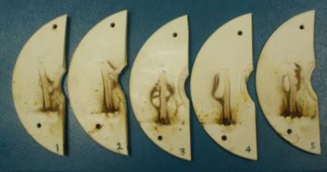
The tracking and erosion test was done for the 5 different brands in the inclined plane test. Figure 5 shows the conventional shape of the specimens that are usually evaluated in the inclined plane test, whereas Figure 6 to Figure 11 show the shape of the specimens evaluated in this work.


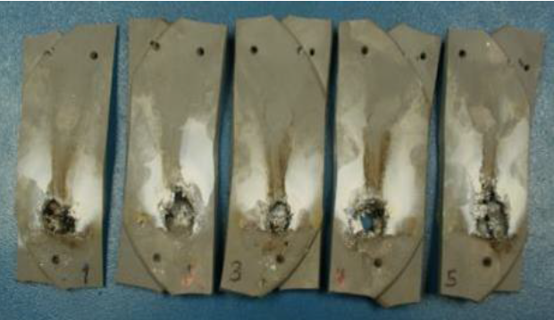


During the test of brand III, the specimens presented perforation in the beginning of the test, this happened in average 14 minutes for the 5 specimens. Due to that, 2 halves of shed were placed one above the other to double the thickness of the specimen and the test was repeated increasing the average time to failure in 108 minutes; Figure 9 shows these specimens after the inclined plane test.
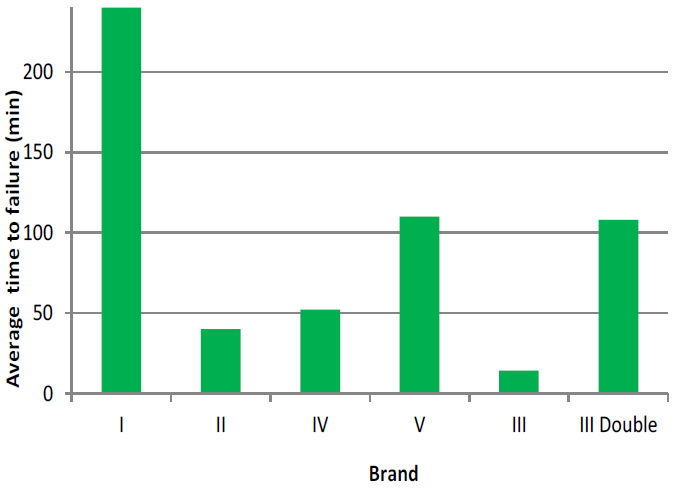
In the case of the inclined plane test, the average time to failure for each brand was registered, this parameter is very important because the brand that has the highest average time to failure is the best brand.
For obvious reasons, the brand that last shorter time is the worst. In Figure 12 is shown the average time to failure for each brand during the inclined plane test.
In the case of the inclined plane test, the average time to failure for each brand was registered, this parameter is very important because the brand that has the highest average time to failure is the best brand. For obvious reasons, the brand that last shorter time is the worst. In Figure 12 is shown the average time to failure for each brand during the inclined plane test.
4.2 Evaluation of Specimens in Laser Ablation Test
In order to corroborate the performance of the different brands of insulators, obtained by means of the fractal analysis of the samples, the same specimens were evaluated by using the laser ablation test [26].
The exposition of the laser beam on the specimen's surface produces molecular vibrations causing the polymer to break down and causes degradation of the material.
At the end of the test, the performance of the specimen is a function of the total eroded mass. Therefore, the specimen presenting the least amount of eroded mass at the end of the test will correspond to the best one.
The results obtained from laser ablation test are shown in Table 1 and in Figure 13.
Table 1 Summary of average eroded mass for three tests of each brand in the laser ablation test
| Brand | Average eroded mass (g) | Standard deviation |
|---|---|---|
| I | 0.0019 | 0.0008 |
| II | 0.0818 | 0.0078 |
| IV | 0.0911 | 0.0008 |
| V | 0.1316 | 0.0158 |
| III | 0.2228 | 0.0101 |

During the test, it was noticed that specimens of Brand I do not absorb the laser radiation because the sample is light brown color and this may be the factor that allowed to have a lower degradation of polymer compared to other specimens.
However, it is important to mention that all tested specimens are of variable grey color, excepting brand I, and it is possible that the specimens do not absorb the same amount of laser radiation. Therefore, it is important to conduct a study of calorimetry, in which we can establish the time of exposure to laser ablation for each specimen depending on its color.
This will ensure that each specimen absorbs the same amount of radiation independently of its color. It is inferable that the laser exposure time will be greater for specimens with light color than specimens with dark color.
4.3 Fractal Analysis Using Commercial Software and New Developed Methodology
Once the image has been processed as indicated previously, it is analyzed by using fractal analysis [25], obtaining a numerical value known as the fractal dimension. For the comparison among brands of insulators, it has been established that the resulting fractal number can be used as an indicator of performance of the insulator.
Table 2 shows the summary of results obtained from the box-counting method using the commercial software FracTop, Benoit 2.0, ImageJ, and HarFA for each insulator evaluated in the inclined plane test.
Table 2 Summary of fractal dimension using commercial software from specimens evaluated in IPT
| Brand | Rubber Type | Fractal Dimension (Ds) | |||
|---|---|---|---|---|---|
| Fractop | HarFA | ImageJ | Benoit 2.0 | ||
| I | HTV | 1.632 | 1.535 | 1.704 | 1.590 |
| II | HTV | 1.699 | 1.651 | 1.745 | 1.673 |
| III | LSR | 1.857 | 1.818 | 1.887 | 1.851 |
| III double | LSR | 1.852 | 1.807 | 1.880 | 1.833 |
| IV | HTV | 1.800 | 1.763 | 1.836 | 1.803 |
| V | HTV | 1.855 | 1.823 | 1.891 | 1.839 |
Figure 14 shows the graph of average fractal dimension for each of the brands by using the four commercial software. Also, for the implemented methods 3D box-counting (3DBC), differential box-counting (DBC), triangular prism surface area (TPSA), and wavelets (WM); the results of the tests conducted for evaluating the performance of the specimens by using directly grey-level images instead of binary images are shown in Table 3.

Table 3 Summary of results obtained for different methods (3DBC, DBC, TPSA, AND WM) using grey-level images
| Brand | Fractal Dimension (Ds) | ||||
|---|---|---|---|---|---|
| 3DBC | DBC | TPSA | WM | ||
| I | 2.093 | 2.121 | 2.346 | 2.595 | |
| II | 2.109 | 2.155 | 2.357 | 2.679 | |
| IV | 2.117 | 2.209 | 2.386 | 2.702 | |
| V | 2.133 | 2.214 | 2.435 | 2.759 | |
| III double | 2.144 | 2.241 | 2.467 | 2.836 | |
| III | 2.149 | 2.244 | 2.474 | 2.812 | |
5 Discussion
Based on the results presented in Table 2, the different brands of insulators can be ranked in 2 ways; this depends on the software used to calculate the fractal analysis, as shown in Table 4. The results are slightly different probably because the variation in the methods that are used to calculate the fractal dimension. Among all the brands of insulators evaluated in this work, Brand III and Brand III double were the only ones that presented perforation, taking into account this fact, it can be established that these brands were the worst ones. In this way, by placing them at the bottom of the ranking, a single ranking table agrees with the performance of the insulators that were evaluated.
Table 4 Performance after IPT ranking by commercial software
| Performance | Benoît 2.0 and Fractop | HarFA and ImageJ |
|---|---|---|
| Best | Brand I | Brand I |
| Brand II | Brand II | |
| Brand IV | Brand IV | |
| Brand III Double | Brand III Double | |
| Brand V | Brand III | |
| Worst | Brand III | Brand V |
As it was expected, the fractal dimension obtained by using directly grey-level images was consistently the lowest one for brand I as shown in Table 3, and it was the highest one for brand III. With the exception of the wavelet method, all methods presented the same behavior. In fact, the resulting ranking is the same as in the case of the evaluation by using binary images.
The same increasing trend is presented for eroded mass obtained by laser ablation test and for the average fractal dimension obtained by using commercial software as shown in Figures 13 and 14 respectively. So, the fractal dimension agrees with the classification by eroded mass.
During the processing of the images there was no way to take into account the depth of the erosion or tracking in the sample, that is, the degradation can only be analyzed on the surface, and the software is unable to assess the severity of the failure based on its depth. In the inclined plane test is considered that the test is finished once that one of the 5 samples presents a failure in the form of perforation or the length of the tracking is 25 mm.
6 Conclusions
The results obtained in this study allow us to establish that the fractal analysis, of tested sheds images, either binary or grey-level analyzed by using commercial software or implemented algorithms respectively, resulted in good agreement with eroded mass and time to failure in inclined plane tests. Further studies involving more brands and more samples are needed in order to determine the difference of using binary images instead of grey-level images. However, it is impossible to fully assess degradation, since this technique only considers the specific area of the tracking but no the depth.
Because of that, the fractal dimension should be contrasted with other test parameters, for example, eroded mass, leakage current, erosion depth, or average time to failure. The obtained fractal dimension should not be considered as the final performance parameter of the specimens tested, but as an addition to a set of parameters to fully analyze the phenomenon of the magnitude of the degradation.
The performance of the specimens undergoing tracking and erosion test is a weighted sum of all aspects involved in the failure. Finally, consistently the best and worst brands of commercial insulators were brand I (less damage) and brand III (more damage) respectively.

