


 text new page (beta)
 English (pdf)
 Article in xml format
 Article references
 Send this article by e-mail
 Cited by SciELO
  Similars in
SciELO
Similars in
SciELO 
 Permalink
1 Introduction
The competitive location models were first introduced by [13]. While [4] proposed the location-allocation problem to locate a set of new facilities to minimize the transportation cost from facilities to customers. This problem was extended to a weighted network [11]. Since then, it has been extensively addressed in the logistics area [2].
When looking for locating facilities in an optimum place, exact optimization models are used, like the Branch and Bound model [9]. On the other hand, when it is enough to locate the new facility in a right place (not the best), heuristic methods are used [19].
The problem of facility location consists in selecting the appropriate geographic location for one or more facilities. There are three different spatial representations: in continuous space, in the network and discrete space. Continuous space allows placing the facilities anywhere within a region [8], in the work of [29] it is used in a model for mixed-integer linear programming.
Differently, in network, it is possible to locate the installations in the periphery or intermediate points of a network as is shown in the work of Serra & Revelle [24,25]. On the other hand, discrete space allows selecting where to locate facilities between a set of possible locations for instance, as it is shown in the work of [23], where it is used for the location of distribution centers for a beverage company selecting among some possible locations.
In the literature, the models of facility location for a new company assume that whoever is going to start a company sets the price and does not care about competition between companies [15], for this reason, many models do not consider the price within modeling.
In some way, it is a hierarchical model where the competitor decides first its locations, and later the company decides locations based on that information.
Many models for facility location start with static competence. Within this model is considered that the existing competition is known, the competition is fixed and the product sold is homogeneous. It also considers that the decisions of the customers when selecting a store are based on the distance to travel, and the unit cost is the same for all the stores. Within this type of problems can be found in the model MAXCAP [22]. This model seeks to maximize the coverage of demand and raises the possibility that one or two stores absorb all demand.
Another problem is the location of competitive facilities with static probability, known as the Huff model [14]. This model has two considerations: i) The attraction that a customer feels towards a store, is proportional to the size of the store, ii) There is a rejection proportional to the distance that customers must travel. This model has been extensively revised and modified. Some authors have given a series of attributes and weights to the facilities to Huff's model [20]. Other authors have added to the Huff model the quality of service, using an exponential attraction [12]. The proposed model seeks to minimize the impact of competition and considers a discrete spatial representation, when analyzing some locations, to establish n facilities. In order to be able to establish value in the competition, square meters of competitive service is used, which is one of the considerations made by the Huff model. This model is one of the most used for the location of retail stores and determines probabilistically the effect of the size and the distance that a customer travels to those facilities [26].
The model also considers a service radius, because there is a maximum time that consumers are willing to travel [1] and customers perceive it as an attractive location regarding distance. In order to feed the model, demand was calculated using the Goodrich proposal [10], which locates the demand from the centroid of a geographical area.
The outline of the manuscript is as follows: In Section 2 a review of models is presented.
In Section 3 the model for the current problem is presented. In section 4, the results of the instances are addressed.
Here, four scenarios are presented, where the first, is the base scenario. The second is used to make the behavior analysis of the competition. The third is used to make the behavior analysis with high demand. The fourth is used to make the behavior analysis to low demand, and the last is the base problem with variations in service radius and in facilities to allocate. In the last section, the discussion and conclusions are presented.
2 Literature Review
There is an extensive literature about facility location, including facility location considering attraction rejection.
According to [16], there are eight criteria to classify the facility location problems, from which this work will be focused on models in discrete space.
The model presented in this paper differs from other models in some of its characteristics, and they will be explained in this section. First, there are models to locate p facilities, like the [5] model, but that does not contemplate the competition and work in the plane or network location at it is done in this paper. Second, some models work with attraction and repulsion, but that only seeks to locate a single installation at a point in a plane [3], in a convex region or a triangle.
The Weber problem: frequency of different solution types and extension to repulsive forces and dynamic processes [27] with two points of attraction and one of rejection, solved by trigonometric methods and do not work with the competition. While the presented model works with locating a set of locations in discrete space with more than two points of attraction and more than one point of rejection, solved with a mathematical model.
Third, the idea of a service radius, attraction and weights are similar to the one proposed by [7] model. They use the sum of the demands of each point of attraction as the weight (W). Also, they use negative weights, and if the sum of all the weights is a positive number, the solution lies in the circle.
In this paper, the weights are positive, and only the customers and competitors in the service radius are contemplated. Fourth, the model of Tellier [28] works with attraction and interaction based on distance, at shorter distance greater interaction, but that model does not work with rejection or service radius.
In the present paper attraction rejection and service, the radius is used. Fifth, there is also cause that population decides to conglomerate in a determined point and introduce centrifugal forces that cause that the population moves away of that point [18].
In that model, the weights are the payment that is given to each worker per unit of work. However, in that case, the attraction is based on the weights given to the jobs differently to the present paper in which the weights are based on the square meters that each competitor has.
Sixth, there is a model that considers attraction and the circular area in order to locate a metropolis [17], but this does not contemplate rejection as the present paper does. Seventh, some works focus on the attraction that a customer feels towards the installations, based on quality and distance [21], but does not work with service radius and rejection as in the present paper. Moreover, in the model proposed by [6], facility location in a network in the presence of competition, and stability concepts are described to define the maximum set of profitable locations that are stable under competition.
According to the reviewed articles, the proposed model differs from others mainly in the attraction-rejection in the base to the square meters of service of the competence, another difference is the particular representation, because the others are located in the plane while the proposed model is located in a discrete space. In addition, differently to a model mention before, which contemplates two attraction points vs. one rejection point while the proposed model contemplates that all the potential customers are attraction points, while all the competitors are rejection points.
Finally, the proposed model contemplates a service radius where the potential facilities provide the service while the analyzed models do not work with this consideration.
3 Attraction-Rejection Model
The model is a mixed-integer linear programming model.
It is considered in discrete spatial representation and considers an influence area, established as a circumference, within which the competition and the possible customers are served. It should be noted that the model is composed of two main parts:
a) One part of the model attracts unsatisfied demand, covering as much demand as possible.
b) The other part of the model rejects competition, moving away from the competitors that mostly affect the facilities.
The model maximizes the profits obtained. It is achieved by getting closer to customers and away from the competition with more impact on the location. For this, the model uses as input data the weights of the competition, the distances of the customers to each of the proposed facilities, distances from competitors to proposed facilities, the service radius and the maximum number of facilities to be opened.
The model considers a service radius because there is a maximum time that consumers are willing to take to travel. It also gives a weight to the competition, according to the square meters of service they have, based on the Huff model.
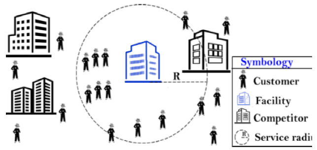
Three potential facilities to be opened are shown in Figure 1. The facilities are affected by competitors and favored by customers. Here, facility j2 is selected to be opened, because it has more customers and fewer competitors.

Although in Figure 1 a simple representation of locations where facilities can be locate-allocate is presented, in real life, with much options of facilities to locate-allocate and many customers to take into account, a model is necessary.
The facility j2 in the real world as is presented in Figure 2. It shows that the radius service is drawing to locate the facility as close as possible to the demand and as far as possible from competitors.
3.1 Mathematical Model
The model needs customer' demands as inputs, customer locations, competitor locations, the service radius, the number of facilities to allocate, the location of possible facilities.
In discrete space models, a group of possible facilities is proposed, and only any of them are allocated to maximize the profits. The following assumptions characterize the model: the customer goes to buy to the nearest company (taking into consideration the distance) within his area. The customer is attracted by the space in m2 of the service area. It is not considered that the price of the products or their characteristics influences the customer.
The model is composed of the objective function (1) and the constraints (2-8).
The objective function looks for covering as much demand as possible and moves
as far as possible from the competition that more affects the facilities. The
first part of the objective function is composed by
Concluding that to less distance more attraction because to less distance more interaction based on Tellier and Sankoff theory [28].The objective function maximizes the demand captured, moving away from the competition that most affects the facilities.
Constraints (2) find that the distance from the customers to the facility is within the service radius. Constraint (3) ensures that at most F facilities are open. Constraint (4), ensure that customers are assigned to only one facility. Constraint (5) ensures that any open warehouse considers its competition. Constraints (6, 7, 8) ensure that these variables are binary. In the model, the next nomenclature is used:
Xij = 1 if customer i is served by facility j, and 0 otherwise.
Ykj = 1 if competitor k is within a service radius of facility j, and 0 otherwise.
Lj = 1 if facility j is allocated, and 0 otherwise.
i =Customer.
j=Facility.
k=competitor.
m=number of customers.
n= number of facilities.
o= number of competitors.
ai=Customer demand.
R=Service radius.
dkj=Distance from competitor k to facility j, where dkj≥1.
dij=Distance from customer i to facility j.
F= Number of facilities to open.
Wj= Weight given per m2 of service of each potential facility j.
Wk= Weight given per m2 of service of each competitor k.
Nkj= Competitor k to facility j in the service radius.
The proposed model is as follows.
Objective function:
constraints:
The model seeks to maximize demand coverage while seeking to distance itself from the competition. The model considers a radius of influence because there is a limit of time that consumers are willing to take to go to the facility. Indeed, this model is giving a weight value to the competition influence, based on the square meters of the service area they have. In addition, the model considers the demand of customers.
In the following sections the determination of the weights of the competition, radius of service, demand, potential facilities, and distances will be explained.
3.2 Determination of Competition Weights
For the determination of competition weights, the Huff model was used. In this case, the square meters of service of the competition were used to calculate the weights, since the M2 of service makes a competitor more or less attractive to customers because the square meters can be used to provide the customer with more services, like, parking, bathrooms, customer service, among others.
To calculate the attraction exerted by each competitor on the customer's equation (9) is used:
Equation 9 calculates the probability Pj that a customer j is attracted towards a facility of competition k and is equal to the number of square meters U that owns the facility of the competitor k, divided by the sum of the M2 of all the facilities of the competition.
It is, the data are taken from three competitors, each of which has 5M2, 3M2 and 2M2, respectively, so the probability of a customer feels attracted to the installation one is obtained using equation (9), as shown below:
Likewise, the probabilities are calculated for the facilities 2 and 3, getting P2=0.3 and P3=0.2, by summing all the probabilities we get 1.
3.3 Service Radius Determination
For the determination of the service radius, it is recommended to consult trustworthy sources for distances in meters that customers usually travel to facilities. Another option is to apply surveys, where the potential consumers of stores were asked about the distance and/or the time they were willing to take to make their purchases and if they usually go walking or in the car or the bus to the facilities.
3.4 Demand Determination
The center of a geographic area could be used to locate the demand [10]. For this, a software of georeferencing is recommended, locating the neighborhoods where the target population live; an example of this can be seen in Figure 3.

The next step is to obtain the data from the population and housing census. In these databases, it can be obtained how many inhabited houses there are in each area, the number of houses multiplied by the amount that the families were willing to spend per week in a commercial center (previously obtained with surveys), to obtain the demand.
3.5 Determination of Potential Facilities
Internet sites where the people can consult rent of commercial areas could be used to locate possible facilities. After locating facilities, the use of a software of georeferencing helped to obtain the longitude and latitude of the possible locations.
The determination of the competition could be obtained in the same way with a software of georeferencing, knowing in advance what kind of companies could compete with the facilities.
4 Model Instances and Results
The mathematical model was solved with LINGO 14 unlimited version; it was installed in a workstation with 4.00 GB RAM, hard drive total size of 1397 GB and Intel (R) Core (TM) i7 - 3770 3.40 GHz CPU processor. In all the scenarios, less than twelve iterations were made by Lingo and less than one second was necessary for each one.
The results obtained with the model are presented. The data used were proposed by the authors based on modified data obtained in a Real instance.
In this section, four scenarios will be presented, the first scenario to establish initial data; the second and third scenarios are presented in order to analyze the behavior of the model to competition; finally, the fourth scenario is to analyze the behavior of the model to low demand.
The presented scenarios are to evaluate the model behavior and to know which facilities allocate in order to obtain the best profit; the purpose is to know if the opening of any facilities will permit to cover more unsatisfied demand.
Scenario 1. For this scenario, there are four competitors (o=4), five customers (m=5), three facilities (n=3), can be opened two facilities (F=2), and the service radius is 500 meters (R=500). The data provided consist on the distances in meters to competitors and customers from the potential facilities, the weights of the competitors are also provided according to the M2 of service area they have plus the service area of potential facilities.
Table 1 presents the distances in meters from the competitors to each of the proposed locations for the facilities. With the data of this table, an analysis of which competitor affects each of the potential facilities to open is made using as parameter a radius of 500 meters, and the results are shown in Table 2, where if the potential facility is affected by competitors a number 1 is used, if it is not, 0 is used.
Table 1 Distances in meters from competitors to each potential facility
| Potential Facilities |
j1 | j2 | j3 | |
|---|---|---|---|---|
| Competitors | ||||
| k1 | 514 | 174 | 80 | |
| k2 | 312 | 458 | 500 | |
| k3 | 180 | 212 | 800 | |
| k4 | 90 | 110 | 300 | |
Table 2 Facilities that are affected by competitors
| Potential Facilities | j1 | j2 | j3 | |
|---|---|---|---|---|
| Competitors | ||||
| k1 | 0 | 1 | 1 | |
| k2 | 1 | 1 | 1 | |
| k3 | 1 | 1 | 0 | |
| k4 | 1 | 1 | 1 | |
Table 2 is shown that facility one is affected by competitors 2, 3 and 4, while facility three is affected by competitors 1, 2 and 4.
Tables 3 and four are calculated in the base to Table 2. For example, for facility one the sum in squared meters of competitors k2, k3 and k4 (which affect the facility) plus the square meters of facility one sum a total of 2081 M2.
Table 3 Square meters and weights for each facility
| Potential Facilities |
j1 | j2 | j3 | |
|---|---|---|---|---|
| Customers | ||||
| M2 | 500 | 700 | 600 | |
| Wj | 0.3367 | 0.3364 | 0.3679 | |
The weight obtained is 0.3364 (700/2081), see in Table 3. Table 4 presents square meters and weights for each competitor.
Table 4 M2 and weights from each competitor to facilities
| Potential Facilities |
M2 | j1 | Wkj j2 |
j3 | |
|---|---|---|---|---|---|
| Competitors | |||||
| k1 | 396 | 0.0000 | 0.1903 | 0.2428 | |
| k2 | 247 | 0.1663 | 0.1187 | 0.1514 | |
| k3 | 350 | 0.2357 | 0.1682 | 0.0000 | |
| k4 | 388 | 0.2613 | 0.1864 | 0.2379 | |
4.1 Analyzing the Behavior of the Model with High Competition
Some changes were made in the distance values from competitors to the potential facilities.
In this scenario, all customers are allowed to be satisfied by any of the three possible facilities and the facilities 1 and three are affected by all competitors.
Scenario 2. The data in this scenario are the same as Scenario 1. There are four competitors, five customers, three facilities, can be opened two facilities, and the service radius is 500 meters.
The distances of the competitors to the facilities are modified, so the facilities 1 and 3 are affected by all competitors; these data are presented in Table 7 and Table 8 presents which potential facilities are affected by the competitors.
Table 5 Record of distances in meters registered from customers to each potential facility and customer demand
| Potential Facilities |
j1 | j2 | j3 | a1 | |
|---|---|---|---|---|---|
| Customers | |||||
| i1 | 1514 | 374 | 120 | 1100 | |
| i2 | 834 | 148 | 240 | 950 | |
| i3 | 439 | 833 | 560 | 500 | |
| i4 | 355 | 788 | 900 | 620 | |
| i5 | 192 | 322 | 800 | 350 | |
Table 6 Customers served by each open facility
| Facilities | j1 | j2 | j3 | |
|---|---|---|---|---|
| Customers | ||||
| i1 | 0 | 0 | 1 | |
| i2 | 0 | 0 | 1 | |
| i3 | 1 | 0 | 0 | |
| i4 | 1 | 0 | 0 | |
| i5 | 1 | 0 | 0 | |
Table 7 Modified distances from competitors to each potential facility
| Potential Facilities |
j1 | j2 | j3 | |
|---|---|---|---|---|
| Competitors | ||||
| k1 | 314 | 574 | 80 | |
| k2 | 312 | 558 | 500 | |
| k3 | 180 | 212 | 300 | |
| k4 | 90 | 110 | 300 | |
Table 8 Facilities that are affected by competitors
| Potential Facilities |
j1 | j2 | j3 | |
|---|---|---|---|---|
| Competitors | ||||
| k1 | 1 | 0 | 1 | |
| k2 | 1 | 0 | 1 | |
| k3 | 1 | 1 | 1 | |
| k4 | 1 | 1 | 1 | |
All customers are allowed to be satisfied by any of the three possible facilities; these data are presented in Table 9.
Table 9 Distances from customers to each potential facility and customers demand.
| Potential Facilities |
j1 | j2 | j3 | a1 | |
|---|---|---|---|---|---|
| Customers | |||||
| i1 | 414 | 374 | 120 | 1100 | |
| i2 | 434 | 148 | 240 | 950 | |
| i3 | 439 | 333 | 360 | 500 | |
| i4 | 355 | 388 | 400 | 620 | |
| i5 | 192 | 322 | 300 | 350 | |
According to the new data, the weights of facilities and competitors are modified as is shown in Tables 10 and 11.
Table 10 M2 and weights for each facility
| Potential Facilities |
j1 | j2 | j3 | |
|---|---|---|---|---|
| Customers | ||||
| M2 | 500 | 700 | 600 | |
| Wj | 0.2658 | 0.4868 | 0.3029 | |
Table 11 Square meters and weights from each competitor to facilities
| Potential Facilities |
M2 | j1 | Wkj j2 |
j3 | |
|---|---|---|---|---|---|
| Competitors | |||||
| k1 | 396 | 0.2105 | 0.0000 | 0.1999 | |
| k2 | 247 | 0.1313 | 0.0000 | 0.1247 | |
| k4 | 388 | 0.2063 | 0.0003 | 0.1959 | |
Once the model has been implemented in LINGO, Z = 1709.44 is obtained, with the option to open facility 2, which is the facility that can serve all customers, as shown in Table 12, and is affected only by competitors 3 and 4, as shown in Table 8.
4.2 Analyzing the Behavior of the Model with High Demand
Demand behavior tests were conducted, establishing a demand of one customer over the other demands by 300%. Only facility 2, which is affected by all competitors, could satisfy the demand of this customer.
Scenario 3. The data in this scenario are the same as Scenario 1. There are four competitors, five customers, three facilities, can be opened two facilities, and the service radius is 500 meters. The data in Tables 1, 2, 3 and four were used.
The demand for customer five is modified to be much bigger than the other demands, and the distance from customer 5 to facility one is modified so that only facility two can satisfy the demand for customer five because the last is within the perimeter of such facility.
The distances of the customers 1, and two are also modified so that their demands cannot be satisfied by facility 2. These modifications are shown in Table 13.
Table 13 Distances from customers to each potential facility and customers demand
| Potential Facilities |
j1 | j2 | j3 | a1 | |
|---|---|---|---|---|---|
| Customers | |||||
| i1 | 1514 | 574 | 120 | 1100 | |
| i2 | 834 | 548 | 240 | 950 | |
| i3 | 439 | 833 | 560 | 500 | |
| i4 | 355 | 788 | 900 | 620 | |
| i5 | 592 | 322 | 800 | 12350 | |
Once the model was implemented in LINGO, Z = 4,783.339 was obtained, with the option to open facilities 2 and 3, where facility two will satisfy the demand of customer five and facility three will satisfy the demands of customers one and two, as is shown in Table 14. Table 15 can be seen that facility two is affected by the four competitors, while facility three is affected by competitors 1, 2 and 4.
Table 14 Customers served by each open facility
| Facilities | j1 | j2 | j3 | |
|---|---|---|---|---|
| Customers | ||||
| i1 | 0 | 0 | 1 | |
| i2 | 0 | 0 | 1 | |
| i3 | 0 | 0 | 0 | |
| i4 | 0 | 0 | 0 | |
| i5 | 0 | 1 | 0 | |
Table 15 Competitors that affect each open facility
| Facilities | j1 | j2 | j3 | |
|---|---|---|---|---|
| Competitors | ||||
| k1 | 0 | 1 | 1 | |
| k2 | 0 | 1 | 1 | |
| k3 | 0 | 1 | 0 | |
| k4 | 0 | 1 | 1 | |
In this scenario, the model seeks to locate the facility closer to the highest demand, regardless of the high competition.
4.3 Analyzing the Behavior of the Model in Low Demand
For this test, all demands are changed in order to be very low, and they are equal.
Scenario 4. The data in this scenario are the same as Scenario 1. There are four competitors, five customers, three facilities, can be opened two facilities, and the service radius is 500 meters. The data of Tables 1, 2, 3 and four are used. The demands are modified and are shown in the last column of Table 16.
Table 16 Distances from customers to each potential facility and modified customers demand.
| Potential Facilities |
j1 | j2 | j3 | a1 | |
|---|---|---|---|---|---|
| Customers | |||||
| i1 | 1514 | 574 | 120 | 35 | |
| i2 | 834 | 548 | 240 | 35 | |
| i3 | 439 | 833 | 560 | 35 | |
| i4 | 355 | 788 | 900 | 35 | |
| i5 | 592 | 322 | 800 | 35 | |
With these data, the model was implemented in LINGO, and Z =47.77 was obtained, with the option to open facility 1 and 3, where facility 1 satisfy the demand of customer 3 and 4, and the facility three will satisfy the demand of customers one and two as shown in Table 17. Table 18 can be seen that facility one is affected by competitors 2, 3 and 4 and facility three is affected by the competitor 1, 2 and 4.
Table 17 Customers served by each open facility
| Facilities | j1 | j2 | j3 | |
|---|---|---|---|---|
| Customers | ||||
| i1 | 0 | 0 | 1 | |
| i2 | 0 | 0 | 1 | |
| i3 | 1 | 0 | 0 | |
| i4 | 1 | 0 | 0 | |
| i5 | 0 | 0 | 0 | |
4.4 Tests of Scenario 1 with Variations
The scenario 1 was modified to analyze the behavior of the model, in Table 19 the results of scenario 1 and its variations can be seen.
Table 19 Scenario 1 and its variations
| Scenario | 1 | 1a | 1b | 1c | |||
|---|---|---|---|---|---|---|---|
| Concept | |||||||
| R | 500 | 500 | 400 | 400 | |||
| F | 2 | 1 | 2 | 1 | |||
| Open facilities | 1,3 | 2 | 1,3 | 2 | |||
| Attended customers | j 1 | 3,4,5 | — | 4,5 | — | ||
| j 2 | - | 1,2,5 | — | 1,2,5 | |||
| j 3 | 1,2 | — | 1,2 | — | |||
| Competitors by facility | j 1 | 2,3,4 | — | 2,3,4 | — | ||
| j 2 | 1,2,3,4 | — | 1,3,4 | ||||
| j 3 | 1,2,4 | — | 1,4 | — | |||
| Z | 1217.84 | 793.59 | 1182.74 | 901.72 | |||
In scenario 1a, only one facility can be allocated. In this scenario, facility two is allocated. This facility supplies customers one, two, and five and it is affected by all competitors. In scenario 1b, the service radius is 400, and two facilities can be allocated. In this scenario, facilities 1 and 3 are allocated. Facility 1 supplies customers 4, 5, and facility 3 supplies customers 1, 2. Facility 1 is affected by competitors 2, 3 and 4, and facility three is affected by competitors 1 and 4. In Scenario 1c, the service radius is 400 m, and one facility can be allocated. In this scenario, facility two is allocated, and it supplies customers 1, 2 and five while it is affected by competitors 1, 3, 4.
5 Results and Discussion
In the paper is shown the way in which the demand is calculated from the population data. The attraction of the competition is established based on the square meters that each competitor owns and the square meters of each facility. A service radius is established according to the distance that customers are willing to travel to go to a facility.
The model analyzes the possibility of opening F-number of facilities, in a finite number of possibilities, establishing a service radius of those facilities, within which are considered customers and competitors that can affect the facilities.
The cases presented had different characteristics. The case 1 was made in order to provide initial data to probe the model, the case 2 was to probe the sensitivity to competition and the cases 3 and 4 were to probe the sensitivity to demand.
In case 1, the result of Z=1217.84 was obtained because the competition will capture part of the market. The solution recommends opening facility one that supplies customers three and four, while facility two supplies customers one, two and five.
In case 2, the competition sensitivity analysis was developed, the distance values of the competitors to the installations were modified, so that installation one, changed from having three competitors to having four competitors, while the facility two, went from having four competitors to having only two competitors, and the facility three changed from having three competitors to having four competitors.
As the result, it was obtained that only opens the facility 2, because this facility provides five customers and only is affected by two competitors, obtaining a result of Z = 1709.44 because the competition will capture part of the market.
In case 3, for demand sensitivity analysis, the demand of customer five was modified, so that the demand of that customer exceeds the other demands over the 300% and only the facility two can satisfy the demand of customer five. It should be noted that facility two is affected by the four competitors.
The solution seeks to open the facility two and three, where facility two supply customer five and facility three supply customers one and two.
The facility three are affected by competitors one, two and four. In this case, a result of Z = 4,783.339 was obtained because the demand is not satisfied for all the customers. In case 4, for the analysis of sensitivity to low demand, the demand of the five customers was modified in order to be a low demand, and all the customers have the same demand.
In this case, the model suggests opening the facilities one and three. The facility one supply customers three and four and facility three supply customers one and two.
The facility one is affected by competitors two, three and four and facility three are affected by competitors one, two and four, obtaining a result of Z=47.77, because of the lower demand and the competitors capturing part of the demand.
In this case, can be observed that the facility two is not open, because all competitors affect this facility. Moreover, in the last test, changing any data from Case 1, it can be observed that the results obtained match when two facilities can be open. Obtaining that the best solution is open facilities one and three.
For other side, when only one facility can be open, always the model suggests open the facility two that is the facility that can supply more demand.
The different scenarios showed that the model is suitable because when all the facilities can supply the customers, the model opens the facility less affected by competitors. When the demand of any customer is very high, the model opens the facility that can provide this customer no matter how much competence can exist in the area. When the demand low and the demand of all the customers are equal, the model opens the facilities with fewer competitors, no matter if the demand is low, the model assigns as much demand as possible. The performance of the model with small instances is good.
6 Conclusions
In real life are required solutions for real problems to cover more customers demand and to consider the competitors are finding the balance between both factors. The proposal considers both factors in order to help practitioners to take logistics decisions. This model is new because no other model considers how a new location is affected by competitors (rejection) and by customers (attraction), both located in a service radio area.
To use the model in order to decide where open a new facility, is necessary to take into account that the result depends on the data that are used to solve the problem and that before to establish a service radius, is needed to determine if the population will go to facilities walking or in the car. Also is necessary to take into account that uses the model with more significant instances could require more time to obtain the solution.
As future work will be sought to make tests with more significant instances and make a comparison with other models, establishing comparatives of time and results and take into account the cost of opening each one of the facilities. Uncertainty in the model can be observed in parameters like customer demand, and the number and location of customers. Other parameters can be analyzed from a scenarios perspective, like the number of facilities to open and the service radius.
These changing parameters can be studied using several techniques like systems modeling, simulations, and stochastic programming. The work presented in this paper shows a limited analysis with the purpose of gaining insight into the model and the effects of some variations. More sophisticated analyses can be considered for future work when more information is available to capture the true nature of variability in those parameters.

