


 nueva página del texto (beta)
 Inglés (pdf)
 Artículo en XML
 Referencias del artículo
 Enviar artículo por email
 Citado por SciELO
  Similares en
SciELO
Similares en
SciELO 
 Permalink
1 Introduction
High-quality depth information is important for many applications, such as 3D scene reconstruction [35], visual odometry [14], action recognition [4,26], scene understanding [21,37], 3D segmentation [9,11], among others. However, specular or light absorbing materials, out of range regions and occlusions produce corrupted depth maps with missing information. These problems are more common in depth sensors that are manufactured with smaller size and lower power requirements but compromising the quality of the data. The most challenging situation arises when unknown regions become large and irregular, affecting considerably the results of the applications.
To overcome these drawbacks we consider the outstanding performance of variational techniques applied to fusion of color images [17] and propose to use them for merging two sources of depth data; one that is noisy and incomplete, coming from the depth camera and the other one that is high-quality data, coming from an optimal 3D model. This model (shape prior) is the one that best fits to its associated depth data in the scene. In this way, we improve the quality of a noisy and incomplete depth map, especially in the region of the object of interest.
The main steps of our system are the following. First, we estimate the optimal model. Second, we place the model using the optimized pose, shape and scale, and read the depth buffer from the current camera pose. Third, we integrate the two depth maps using variational techniques. These steps are intended to serve as a pre-processing stage for the aforementioned applications, specially for 3D scene reconstruction.
We can outline three main contributions: 1. We propose an approach to enhance depth maps by integrating depth measurements and shape prior data using a novel formulation of an objective function with a variational approach; 2. The object pose optimization is solved using Lie algebra se(3) instead of the group of rigid transformations in 3D space, SE(3); 3. We quantify the accuracy of pose, shape and scale optimizations. Moreover, we compute the completeness and accuracy of inpainted and denoised depth maps.
This work is structured as follows. In section II similar works are presented. In section III the main processes carried out by the system are described: model alignment, truncated signed distance function TSDF estimation, model compression, dimension reduction, estimation of the optimal pose and scale, search of the optimal latent variable, and integration of the optimal model with a novel variational method. In section IV experiments for optimizing pose, scale and shape with synthetic and real data are carried out. Moreover, experiments for quantifying the accuracy of the enhanced depth maps are described. Finally, the conclusions are presented in section V.
2 Related Work
Techniques for depth recovery include morphological filters [32], Laplace filters [23,33], Markov Random Fields [27], multilateral filters [13,22], non-linear diffusion and variational frameworks [7,10,28] and learning-based methods [12,19,34]. Our system presents a novel approach motivated by outstanding works in object shape priors, scene shape priors and variational techniques. Next, we describe some details about these systems and we compare them with ours.
The system [30] is the first one that back projects depth images and evaluates the resulting point cloud in a 3D level-set embedding function that represents an object model implicitly, instead of projecting the model to the image plane and measuring the discrepancy between expected image cues and the observed ones. Moreover, no point correspondence is required, unlike Iterative Closest Point ICP, since the alignment consist in evaluating the closeness of the points to the zero-level of the embedding function. The authors in [18] remove point cloud artifacts like noisy points, missing data and outliers using a learned shape prior of an object of interest.
They use the discrete cosine transform DCT for compressing the SDF values and GPLVM for dimension reduction.
The system [1] learns a semantic prior comprised of a mean shape for a category (common aspects in shape of a category) and a set of weighted anchor points for instances of the category (specific details). The augmented reconstruction consists in matching anchor points (HOG features), warping by anchor points (an extension of thin-plate spline transformations [31]) and refinement. The system [6] combines shape priors and live dense reconstruction using a monocular camera. Photo-consistency and a variational approach are used for building depth maps [25] that are fused for creating a dense reconstruction, PTAM [16] for tracking the camera, a part-based object detector [8], and GPLVM to represent shape priors. The energy function, besides depending on the evaluation of the 3D points on the embedding function like [30] and [18], depends on the matching between the 2D object segmentation, defined by the foreground and background, and the projected 3D SDF.
The system [29] estimates depth maps using a monocular camera in workspaces with large plain structures like floors, walls or ceilings. Good depth data is propagated to an interior pixel (inpainting) from the closest valid pixels along the main 8 star directions by using a non-local high-order regularisation term, in a variational approach, that favours solutions with affine surfaces (prior). The energy is minimized in straight way with the primal-dual algorithm. The system [5] includes a term, besides the data term and regularization term, that depends on three scene priors: planarity of homogeneous color regions (using superpixels), the repeating geometry primitives of the scene (data-driven 3D primitives learned from RGBD data), and the Manhattan structure of indoor rooms (layout estimation and classification of box-like structures).
Our system is not based on scene shape priors like [5,29] but on object shape priors like [1,6,18,30]. However, it does not uses neither anchor points like [1] nor a depth and intensity-based energy function like [6], but GPLVM like [6,18] and a depth-based energy function like [18,30].
We use a variational technique, like is done in [5,29] for merging scene shape priors, but we exploit the idea of integrating two depth maps, one coming from the sensor and the other one coming from the object shape prior, in a similar way as is done for aerial color images in [17]. The latter system transforms a large point cloud into a common orthographic aerial view. This noisy color image with undefined areas due to occlusions and non-stationary objects is subjected to denoising and inpainting by integrating redundant observations of the same scene using variational techniques. It uses the primal-dual algorithm for minimizing the proposed energy. Finally, our approach implies that, in a future work, the enhanced depth maps will be fused instead of including directly the shape prior as a volumetric structure into the general reconstruction of the scene like is done in [6].
3 Methodology
The main pipeline of the system is shown in fig. 1. The set of reference models (predefined database of cars) are aligned using ICP for getting models with the same scale, translation and rotation. A volumetric grid with TSDF values is computed and a compression is done using DCT, for maintaining just the low-frequency components of the reference models. A continuous, nonlinear, probabilistic and lower dimensional latent shape space that captures the prior knowledge on the 3D shapes that an object can take is found with Gaussian Process Latent Variable Models GPLVM.

Scaled conjugate gradient SCG is employed for leaning the mapping between the latent variables and the low-frequency components (coefficients). Next, the optimal pose, scale and shape are computed and the coefficients associated to the latent variable that best fits to depth data are estimated. The 3D level-set embedding function encoded in the coefficients is computed with the inverse discrete cosine transform IDCT. The optimal model is used for creating a synthetic depth map by reading the depth buffer of the explicitly represented model seen from the estimated camera pose.
The synthetic depth map is merged with the depth data coming from the sensor using a novel variational formulation. In the next sections, the main modules of the system are explained.
3.1 Alignment and TSDF Estimation of the 3D Models
We downloaded 49 models of cars from Turbosquid, a vast online catalog of 3D models. We align each model w.r.t a base model (see fig. 2(h), model chosen arbitrarily) using just the vertices of the triangular mesh, read from an .obj file. Initially, the point cloud of the base car is translated from their center of gravity to the origin. Then, it is scaled for fitting it to the volumetric grid, and the average distance of each point to the new origin is computed (see [3] for more details):

Fig. 2 9 of the 49 3D models of instances of the class car (object of interest), used for estimating the latent space
where Nbase is the number of points of the base model. The same process is carried out (translation and average distance computation) for the point cloud of the model i for getting si. The scale is computed as:
This scale is applied to model i in order to get models with the same size. Then, the models are manually oriented in such a way that their frontal sides point to the same direction, standing over a parallel supporting plane. This initial alignment is refined using ICP, implemented in CloudCompare.
Once the models have been aligned, the model i is loaded in OpenGL using the vertices and facets (just geometry data), creating a continuous surface. The virtual camera is moved in such a way that circular and vertical scanning at different longitudes (changes in azimuth and elevation of 10°) are performed.
The optical axis of the virtual camera is always pointing to the origin that
coincides with the center of gravity of the loaded model. Depth images, obtained
by reading the depth buffer of OpenGL, are fused into a volumetric structure,
storing in each voxel a TSDF value. We have
Nm= 49 3D models of cars with
different shapes (see 9 of the 49 models in fig.
2). Each model is a 3D level-set embedding function defined by a
volumetric grid of Ng ×
Ng × Ng voxels, with
Ng = 128. The matrix
3.2 Compression of the Embedding Function
The DCT transforms a time domain signal to a frequency domine signal. It is used
for compression of audio (e.g. MP3) and images (e.g. JPEG) where small
high-frequency components can be discarded. We use here this technique for
compressing the TSDF values of the volumetric grid. Let
where α(v,w)=αv(v)*αw(w), with:
Since we have Ng = 128 slices, the size of ϕi is (Ng × Ng). Equation (3) can be expressed as matrix and array multiplications:
where
We extend it to the three-dimensional DCT and apply the property of separability (see [15] for more details), computing the 3D-DCT in two steps with 2D transformations over the slices for each i along dimension u and a final 1D operation. Figure 3 shows the 3D models obtained using 10, 25, 35, 50, 75 and 100 coefficients of the model visualized in 2(b). Here we can see that the information about the general shape is stored in the low-frequency components and the fine details are store in the high-frequency components.
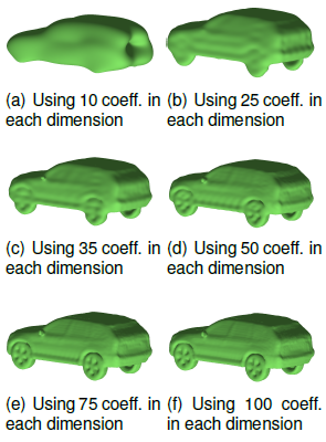
Fig. 3 3D model of fig. 2(b) using different number of coefficients in each dimension (degree of compression)
Note that for 50, 75 and 100 coefficients there are not significant changes in appearance. We consider that 25 × 25 × 25 coefficients are enough for our purposes (like in [18]).
3.3 Learning the Latent Space
The Latent variable Model LVM is used for dimensionality reduction, to capture
the shape variance as low dimensional latent shape spaces, such that the
resulting latent variables have less dimensions than the original observed data.
Let
Let
Since the mapping χj→
Yj is modelled using a Gaussian process, we
can define areas of high probability, it means, areas where there are high
certainty of getting a valid shape. Moreover, this technique allows to map
coefficients from a continuous latent space (no just the ones used for
learning), creating a continuous search of the latent variable that best fits to
data. We define the vector
It is the vector of parameters that solves the following optimization problem:
where Nm is the number of models, K
is the covariance matrix which is estimated with a Kernel function, and
where δij is the Kronecker delta function. We initialize the latent variables of the vector of parameters W with the estimation got with Dual Probabilistic PCA. Then, we use the scaled conjugate gradient SCG algorithm for refining the initial estimation. It combines the model trust region approach, known from the Levenberg-Marquardt algorithm, with the conjugate gradient approach.
The pseudocode and more details about SCG can be found in [24]. The parameters for the kernel are set according to [20]; θ1 = 1, θ2 = 1, θ3 = exp(-1), and θ4 = exp(-1). With these values we can set the initial kernel and continue the iterative process until convergence.
The resulting latent space is employed in section 4.1 for shape optimization. Besides the mean value, each point χP in the latent space has a variance which is computed as:
The parameters for mapping converged to θ1 = 10.4195, θ2 = 1.6784, θ3 = 84.5378, and θ4 = 1.1679.
3.4 Shape Prior Estimation. Shape Optimization
We define an energy that depends on the sum of squared residuals:
where the residual vector Φ is defined with the German-McClure function, which is robust to outliers:
where σ is a constant parameter, Xq =
[XqYqZq]
is one of the Np 3D points that are evaluated (3D
interpolation) in the embedding function ϕ. Points that are
back-projected outside the volumetric grid are assigned a large value. The
derivative of the energy w.r.t. the latent variable
The first term on the right is the residual vector Φ. The variations
of the residual vector Φ due to changes in the latent variable
where:
For defining the second term on the right of eq. 13 we express the embedding function ϕ in terms of the latent variable:
The function IDCT(·) is the inverse discrete cosine transform applied to the mean
v of the coefficients associated with the
latent variable
Considering that the derivative of the IDCT of a variable is the IDCT of the derivative of the variable, we have:
where:
We start with α = 1e - 4. After each iteration, the new energy is compared with the previous one. If the energy has decreased, α is reduced by a factor of 10 and the parameters are updated. If the energy has increased, the parameters are not updated and α is increased by a factor of 10.
3.5 Shape Prior Estimation: Pose and Scale Optimization
We now differentiate the energy of eq. (10) w.r.t. the pose and scale, optimizing
them in separated and alternating way. The pose is minimally parametrized with a
vector
Again, the first term on the right is the residual Φ. The variations of the residual vector Φ due to changes in pose ζ correspond to the Jacobian for this problem:
The first term on the right was defined in equation (14). The second term on the right is:
Since a point Xq = [XqYqZq] (coordinates of voxels referenced to the initial coordinate system q), we get:
with h = 10-8 for all the components. For defining
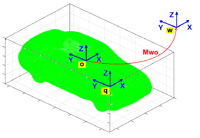
Mwo is the transformation matrix between the object and the world system. Moq is the transformation matrix between the initial and the object system. It corresponds to a translation to the center of the volumetric grid. Figure 4 shows the initial coordinate system q, the object system o, and the world system w. Since the point cloud is referenced to the world coordinate system, the 3D model is also referenced to this system and then, aligned with the point cloud.
S scales the points Xo and is defined as:
Solving for the point Xq, we get:
The transformation matrix Mow is updated as:
where the incremental change in the transformation is expressed using the exponential mapping and the lie algebra:
The operator [⋅]x transform a six-elements vector to the skew matrix:
Δζ is computed in similar way as
where the derivative of the exponential w.r.t the first element of the vector ζ is:
This derivative is a generator for rotations in x-axis in the lie algebra. The same process is carried out for the remaining five parameters. Multiplying by the homogeneous form of Xo and organizing, we get a 4 × 6 matrix.
Following a similar process for scale optimization, we consider the parameters of pose constant and derive Xq from eq. (27) w.r.t the scale parameter:
where
3.6 Inpainting and Denoising
TV-based methods are well suited for tasks like depth data integration, as was probed in [36]. In our context, an energy defined by a TV-based regularization together with a data term that measures the discrepancy between two sources of data (the depths coming from the model Dm(μ) and from the sensor Ds(μ)) and the sought solution Df(μ), is implemented:
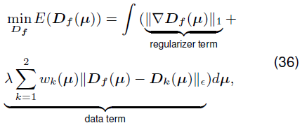
where λ defines the balance between the regularizer term and the data term, D1(μ) = Ds(μ), and D2(μ) = Dm(μ). We apply the robust Huber norm over the data term where:
The
where w(μ ) = 0 corresponds to pure inpainting at location μ . In consequence, the regularizer term allows smooth solutions and the data term allows solutions similar to the depth sources. The energy defined in eq. (36) is minimized using a first-order primal-dual algorithm.
3.6.1 Primal-Dual Algorithm
The regulariser and the data term of eq. (36) can be written in a more general form:
In our case,
where ϱ and rk are dual variables
associated to the primal variables y and
φk respectively, and
where
where
Following the algorithm 1 of [2] and the parameter setting of
[17]
we set the primal and dual time steps with τ = 0.05 and σ = 1/(8τ),
respectively. The Huber norm parameter
Based on [2], the iterative optimization corresponds to perform in alternating way gradient ascent over the dual variables and gradient descent over the primal variable, projecting the results onto the constraints and updating the primal variable, as is summarized next:
where A* is the adjoint operator of the gradient operator and corresponds to the
negative divergence operator,
4 Results
For testing our optimization algorithms when one of the three variables is unknown (shape, pose and scale) we use a down-sampled point cloud coming from the vertices of the triangles computed with the marching cubes algorithm for the compressed version of the base model (fig. 2(h)).
When shape, pose and scale are unknown, we test our algorithms with data coming from the kinect 1.0 and with synthetic data got from a 3D scene. For these experiments we also carry out depth integration using our proposed variational formulation and quantify the completness and accuracy of the enhanced depth maps.
4.1 Results in Shape Optimization
The goal is to refine the shape associated to an initial latent variable in order to reduce the residual computed by evaluating the current embedding function in the point cloud (eq. (10)). In this experiment, the pose and scale are considered known. Figure 5(a) shows an explicit representation of the model for the initial latent variable.
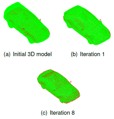
Fig. 5 Evolution of the shape in the optimization process. The search is done in the latent space and the model is obtained with the inverse DCT. It takes 15 iterations for converging. The model is drawn in green and the point cloud in red
Figures 5(b) and 5(c) show the model for iterations 1 and 8, respectively.
Figure 6 shows the path of the
iterative search in the latent space. It starts with a latent variable

Fig. 6 Latent Space with the 49 latent variables (in black) used for learning the mapping parameters. Low variance regions are drawn in blue while high variance regions are drawn in red. More likely valid shapes are obtained in blue areas. The green point is the ground truth in latent variable. The search path of the latent variable that best fits to data is drawn in orange. The resulting latent variable is drawn in dark orange
The Euclidean distance between the estimated latent variable and the ground truth decreased from 0.9551 in the initialization to 0.1122 in iteration 15, getting a reduction in error of 88.25%.
4.2 Results in Pose Optimization
In this experiment the shape and scale are considered known and an initial pose is refined in order to align the embedding function with the point cloud. The ground truth in position is the origin and in orientation is the identity matrix. The initial position is two = [-0.2 0.2 0.2] with an Euclidean distance to the origin of 0.3464. The initial orientation corresponds to a rotation of αz = - 30 around z-axis w.r.t the ground truth.
Figure 7(a) shows the initial pose, while fig. 7(b) and 7(c) show the pose for iterations 20 and 50, respectively. The evolution of the Euclidean distance from the model to the origin and the evolution of the model orientation w.r.t. the ground truth are presented in fig. 8(a) and 8(b), respectively. The orientation Rwo is represented with rotations over the fixed axis x, y, and z (in this order).

Fig. 7 Evolution of the pose of the embedding function in the optimization process. The model is drawn in green and the point cloud in red
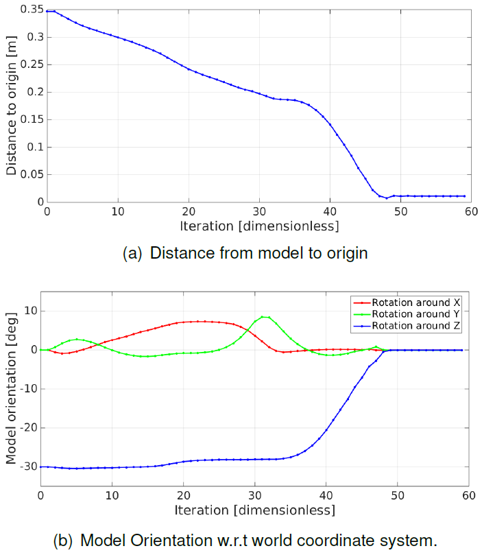
Fig. 8 Evolution of the position and orientation with respect to the ground truth. It takes 59 iterations for converging
The final position is two = [0.0032 -0.0104 0.0035] , with an Euclidean distance to the origin of 0.0114. The final orientation is αx = -0.0017o, αy = -0.0663o, and αz = -0.0209o. It converges at iteration 59, achieving a reduction in position error of 96.70% and in rotation around z-axis of 99.93%.
4.3 Results in Scale Optimization
For scale optimization, the shape and pose are considered known. Recall that the same scale is used in the three dimensions. The initial value in scale is s = 0.4. The ground truth in scale is s = 1.0. Figure 9(a) shows the model with the initial scale (s = 0.4), meanwhile figs. 9(b) and 9(c) show the model with the scale of iterations 1 (s = 1.5855) and 10 (s = 1.0053), respectively. The error for iteration 10 is 0.53% of the ground truth. The reduction in error is 99.12%. Figure 10 shows how the scale gets close to the ground truth (s = 1.0).
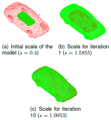
Fig. 9 Evolution of the scale of the embedding function in the optimization process. The model is drawn in green and the point cloud in red

4.4 Results in Pose, Scale and Shape, with Real Data
Now, we use a point cloud coming from a depth map taken with the Kinect V1 of Microsoft. The Kinect was moved by hand in front of a toy car while VGA images were captured at 30fps. We selected one depth and intensity image (see figs. 14(a) and 14(b)) and manually segmented the toy car, getting the mask of fig. 11(a). The resulting 3D points Xr associated to the segmented car (red points in fig. 11(b)) are referenced to the camera coordinate system, where the z-axis is perpendicular to the image plane.

Fig. 11 a) Mask of the segmented car. b) Point cloud associated to the segmented region (lateral side of the toy car)
Then, we compute 3D points referenced to the world coordinate system,
Xw =
MwrXr, where
Mwr is a rotation of 90° around the
y axis followed by a rotation of -90° around the new z
axis. As was doing for model alignment in section 3.1, the point cloud of the
toy car referenced to the world system Xw is
translated from its center of gravity to the origin
The initial position of the car is defined as the center of gravity of the point cloud referenced to the world coordinate system, adding 4% of the x-component (z-axis in the camera coordinate system) to itself since the data belongs just to a side of the whole car:
As in [6], we assume that the toy car is over a flat surface, so computing the normal of this surface allows us to estimate an initial orientation of the car. This process begins by calculating 3D points for pixels in a region bellow the segmented area which belong to the supporting plane. Then, RANSAC is applied: three points are randomly selected and the parameters that define a plane are computed.
The points that fulfill with the computed plane (under a threshold) are counted. The random selection process was repeated 100 times and we chose the parameters that generated the largest number of inliers (points under a threshold when the plane is evaluated).
The resulting normal n , shown in figure 11(b), is used for computing two angles α and β that moves the embedding function to the supporting plane:
The transformation consists of a rotation of -α over the y-axis followed by a rotation of β over the new x axis. The third angle γ needed for totally defining the orientation of the embedding function is the rotation around the unit normal (new z axis). This angle is found through exhaustive search with α between 10° and 360° and with an increment of 10° ; the selected α is the one that produces the minimum energy when eq. (10) is evaluated. Finally, the initial transformation matrix Mwo is:
with
For comparing this orientation with the final one, we use rotations over fixed
axis, x, y and z (in this
order), with αx = 9.1136°, αy = -18.0095°, and
αz = -21.0621°. The initial scale is s = 0.1571,
and the initial shape is the one associated to the reference model employed in
the model alignment process
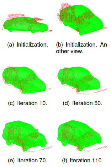
Fig. 12 Evolution of the pose, scale, and shape of the embedding function in the alternating optimization process, for real data using the Kinect. The point cloud is drawn in red
For this test, we carry out two cycles with the sequence: 20 iterations for pose
and 5 iterations for scale. At the end of this sequence, 50 iterations have been
done and very close pose and scale estimations are obtained (see 12(d)). With these estimations we can
perform exhaustive search over the Nm = 49 models of
cars used for learning the latent space. The latent variable with the 3D level
set that produces the minimum energy
The final scale is s = 0.1602, and the final latent variable is
Figure 13 shows the evolution of the energy, drawing with red, green, and blue the pose, scale and shape optimization, respectively. The synthetic depth map got by reading the depth-buffer of OpenGL from the current camera pose is presented in fig. 14(c).
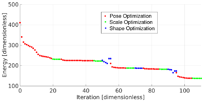
Fig. 13 Evolution of the energy for pose, scale, and shape optimization, in alternating way, using Levenberg Marquardt and the Kinect V1
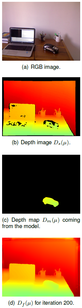
4.4.1 Results in Inpainting and Denoising
Since the main goal is to reduce noise and complete missing data in the depth
map, especially in the region of the car, we get depth data of the optimal 3D
model seen from the real camera pose. Figure
14(b) shows the depth map coming from the sensor while fig. 14(c) shows the depth map coming from
the optimal 3D model. Note that the former image has missing data due to
possible dark, very reflective and translucent objects, out of range objects or
occlusions. The last image has defined data just for the 3D model.
Figure 14(d) shows the sought solution got with the optimization process for iteration 200. Note that the filled areas are smooth and undetectable, achieving a real appearance. The inpainting in the top and right side of the depth map is not so good since there is not data neither in Ds nor Dm and the missing data covers large areas.
We analyzed the performance of the inpainting and denoising algorithm using a slice around the x-axis (see fig. 15). Note that missing data stays mainly in the image borders, in the laptop region and in the car region (inside the vertical lines in fig. 15). It is 22.81% of the total amount of data in the slice.

Fig. 15 Depth map denoising and inpainting using shape priors and variational techniques along a slice. The vertical lines encompass the car
The solution remains similar to the sensor data but it fills missing data, integrates depth data coming from the model, is smooth but preserves discontinuities. Evaluating the completeness of the car, we can state that the algorithm fills 33.28% of missing data. This estimation was done for pixels belonging to the segmented area of the whole car.
4.5 Results in Pose, Scale and Shape with Synthetic Data
For this experiment we have created in Blender a 3D scene composed of a floor, a desk, a car, a mug and a lamp. A depth map (see fig. 17(f)) and a rgb image have been rendered from the virtual camera. The depth data is in the range [1.2045 8.9610]m. We added Gaussian white noise with SNR of 5dB to the rgb image (see fig. 17(a)) and 30dB to the depth map. Moreover, we simulated missing data in the depth maps with rectangles of 40 × 20 pixels containing nans, randomly placed in the depth maps. The percentages of missing data that we used were 23.65% and 40.02% (see figs. 17(b) and 17(g), respectively).
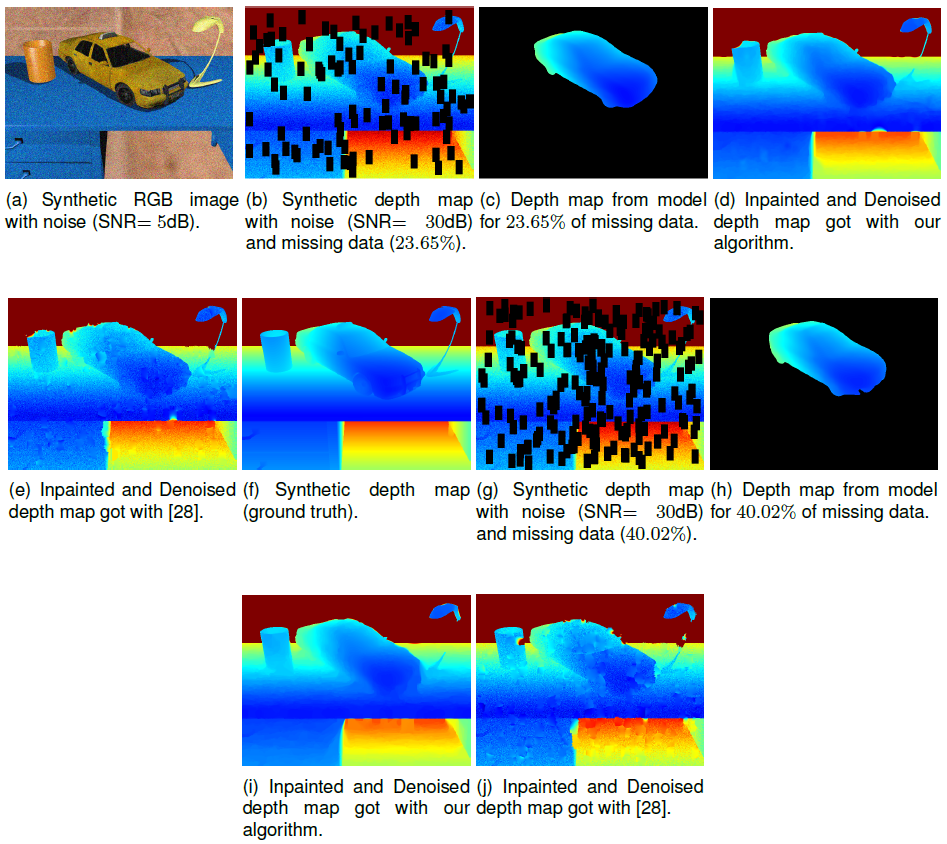
Fig. 17 The first figure in the first and second rows are the rgb image with noise and the ground truth in depth. For the remaining figures the first row contains images for the depth map with missing data of 23.65% while the second row for the depth map with missind data of 40.02%. From left to right: depth map with noise and missing data, depth map coming from the optimal model, our results, results using [28]
The process for estimating the optimal shape prior (initial estimation and the iterative refinement) and for getting a depth map of this model is similar to the one carried out previously for real data. Figures 16(a) and 16(b) show the aligned models with the point clouds for 23.65% and 40.02% of missing data, respectively.
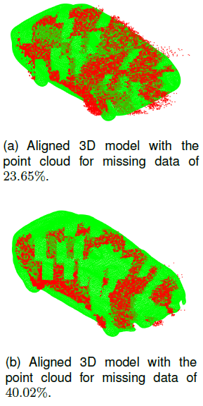
Fig. 16 Results of the aligment process between a 3D-level set and the point cloud. a) For depth map with missing data of 23.65% and b) For depth map with missing data of 40.02%
Our algorithm performs 500 iterations for the depth map with 23.65% of missing data and 700 iterations for the one with 40.02%. We compare the results with the ones obtained with the outstanding system of Pertuz and Kamarainen [28], employing their code publicly available.
It uses anisotropic diffusion and a region-based approach for inpainting sparse depth maps. Table 1 shows that our algorithm outperforms [28] for both percentages of missing data. In fig 17 we can see that the inpainted and denoised depth map got with our algorithm is smoother and preserves discontinuities in a better way than [28]. We did not use more percentage of missing data since it affects the alignment of the model, producing incorrect estimations of the optimal model.
4.5.1 Time
Our system for inpainting and denoising runs on a laptop Hewlett Packard with a processor Intel Core i7-2.2GHz, 11.7GB of RAM memory, a graphic processor NVIDIA GEFORCE 755M and Ubuntu 14.04 as operating system. OpenCV is used for processing images, Eigen3 for matrix operations, OpenGL for drawing the 3D model and getting depth information from it, and Cuda 7.5 for speeding up the algorithm for merging the depth data coming from the sensor and from the optimal model.
The algorithm for estimating the optimal model was implemented in Matlab. Table 2 shows the average on processing time for the main processes. The implementation on GPU of the algorithm for estimating the optimal model is left for future work.
Table 2 Processing time for inpainting, denoising and merging
| Process | Time[ms] |
|---|---|
| First line of eq. (47) | 6.501 |
| Second line of eq. (47) | 5.373 |
| Third line of eq. (47) | 3.247 |
| Remaining processes | 0.573 |
| TOTAL ITERATION | 15.694 |
The algorithm takes 7.847s (500 iterations) for the depth map with 23.65% of missing data and 10.96s (700 iterations) for the depth map with 40.02% of missing data.
5 Conclusion
We have developed a system that optimizes a 3D model, represented as a 3D level-set embedding function, w.r.t. pose, scale and shape and uses depth data of the optimal model for depth denoising and inpainting of a raw depth map coming from a depth sensor, achieving significant results in completeness, specially in the area associated to the object of interest that has a high percentage of missing data. The results have been satisfactory.
First, the embedding function was successfully compressed from 1283 to 253 DCT coefficients (compression ratio of 134,22) and reduced from 253 to 2 dimensions (bi-dimensional latent space) using GPLVM, for a more efficient search of the optimal model.
Second, the optimization was outstanding: the shape optimization converge in 15 iterations with a reduction in error of 88.25% w.r.t. the initial estimation; the pose optimization converge in 59 iterations achieving a final error in position of 1.14cm and less that one tenth of degree in rotation around each axis (reduction in position error of 96.70% and in rotation error around z-axis of 99.93%) validating our proposed technique based on Lie algebra; the scale optimization converge in 10 iterations, getting a final error of 0.53% of the ground truth (reduction in scale error of 99.12%).
Third, the inpainting and denoising process using variational techniques achieved a significant increase in completeness of the depth map coming from the Kinect 1.0, filling 32.28% of missing data of the segmented region of the car, smoothing the data but preserving discontinuities. Moreover, the accuracy of the enhanced depth maps got from synthetic depth maps with 23.65% and 40.02% of missing data is higher than the one obtained with the outstanding algorithm for depth recovery [28].
For future work we will use shape priors and depth integration with variational techniques for enhancing the quality of depth maps built with a monocular camera and we will fuse them into a volumetric structure for getting an improved dense reconstruction.

