


 text new page (beta)
 English (pdf)
 Article in xml format
 Article references
 Send this article by e-mail
 Cited by SciELO
  Similars in
SciELO
Similars in
SciELO 
 Permalink
1 Introduction
Now-a-days Micro-Electro-Mechanical Systems (MEMS) technology allied with wireless communication technology together has invented the small sized sensor nodes that are very economical and are very well organized to sense, evaluate and collect data from a particular environment. Even though the sensors are driven by battery power with limited quantity of processing speed and memory, they are capable of sensing or transmitting data. As the sensors can be installed very close to the monitored incident, chances of getting excellent quantity of accurately sensed data becomes higher. Since its inception, the role of a WSN in various security and surveillance related application is growing enormously.
Apart from security issues, WSN is also applicable in disaster management [34,33], habitat monitoring [21], waste management [43], endangered species tracking [2], health monitoring [13,30], intrusion detection [35] etc.
From the very beginning of research in the field of WSN, coverage has got the highest priority, especially area coverage [7]. Coverage denotes whether every point inside the Region of Interest (ROI) is sensed by at least one sensor or not. In the problem of coverage, each sensor has to enfold some sub-region and summing up the entire covered sub-regions, one can have a totally covered region in the WSN.
As the nodes are deployed randomly in the ROI, some area gets dense deployment of the node while others get sparse deployment. Due to the sparse node deployment, some region may fall short of coverage and results a coverage-hole.
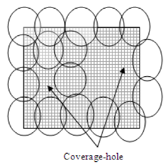
While discussing about the node deployment, it is assumed that the sensing field will exclusively be covered with sensors. But if we see practically just like figure 1, there may be several coverage holes, which are the areas not being covered by any sensor.
There are lots of reasons behind the creation of coverage-hole. Other than random deployment of nodes, incorrect network topology [24], replacement of node [39], presence of obstacle in the ROI [12], unfriendly environment and drainage of power [37] also develops coverage-hole. Therefore, the detection of such coverage-holes is very essential [6] as the presence of holes can degrade the performance of a WSN in terms of weak communication, additional energy consumption and loss of valuable data.
In a WSN, due to random deployment, there can be two types of nodes, the external nodes - those take part in the boundary formation and the internal nodes - those do not contribute to any boundary. The external nodes take active part in security & surveillance related tasks whereas, internal nodes might be useful in routing job. Again, the nodes representing the boundaries can be of two kinds. One represents the hole-boundary and the other representing the network-boundary as shown in figure 2.

The network-boundary nodes encircle the ROI of the whole network and the hole-boundary nodes enclose the region in the ROI where sensing or transmitting is not possible. Generally, hole-boundary is composed of the nodes which are out of functions [39] and the presence of hole in the network is identified by the hole-boundary nodes those isolate the holes from the covered region.
Even from the internal nodes, the nodes which are not functioning can contribute to the existing hole-boundary nodes or can formulate a new hole. Therefore, the identification of hole-boundary is important due to the following reasons:
— Hole-boundary can accurately identify the non-functional nodes.
— Detection of hole-boundary can prevent data loss in the network by efficient routing.
— Identifying hole-boundary can compute the hole-area accurately.
— Hole-boundary improves [41] geographic multicasting.
— Proper detection of hole-boundary can estimate the number of extra node required for hole-healing.
In this paper, many issues related to hole-boundary detection have been incorporated based on recent literature. The objectives of this paper are:
— To present a wide-ranging review of the very recent hole-boundary detection algorithms.
— Provide a categorization of the different hole-boundary detection algorithms for easy understanding.
— Analyze the features, advantage and disadvantage of each algorithm for future reference.
— Present a comparative study on the algorithm's performance as claimed by the authors.
— Raise a few research queries related to hole-boundary detection for future direction of work in the field of WSN.
The rest of the paper is organized as follows: Section 2 describes the preliminaries required for hole-boundary detection; Section 3 depicts category-wise various boundary detection algorithms in details; Performance analysis & Summarization is done in Section 4; Section 5 reflects various research queries identification and finally, Section 6 concludes the paper.
2 Preliminaries
In this section, a rapid discussion is done about the network model and few terminologies or definitions required for explaining the various hole-boundary detection algorithms.
2.1 Network Model
In this paper, we have made a few assumptions required to describe the network model. Let us first assume that the WSN is represented by a connected graph G(V,E) where V = S1,S2,...Sn be the set of n sensor nodes and E is the set of connectors between those nodes. Additionally, the following assumptions are also there:
— The deployment of the sensor nodes in the ROI can be of deterministic[9] or random[5]. In a friendly and controlled environment, deployment can be deterministic whereas, random deployment is preferable in harsh environments.
— The 2D ROI may be of shape rectangular[25] or convex [19] containing homogeneous[18] nodes. Sometimes mobile nodes [36] can also accompany the static nodes.
— All nodes within the WSN have the same sensing radius, RS and communication radius, RC. Based on requirements, the relation between the two can be of: in [19] RC > 2RS, in [44] RC = RS and in [25] RC = 2RS.
— A unique node ID is sipplied to each node.
2.2 Node Location Information
The node location information is treated as a prerequisite in hole and boundary detection algorithms. Among all the positioning techniques[29], Global Positioning System (GPS)[10] is the most accurate location finding measure. In adverse situations if GPS is inaccessible, then ToA [15], AoA [32], TDoA [3] and RSSI Profiling [31] can be used to detect the node location.
2.3 Definitions
This subsection contains the following definitions used in different algorithms for hole-boundary detection:
2.3.1 Active Node (AN)
A node participating in data reception and transmission is known as an active node and is shown in figure 3.

2.3.2 Redundant Node (RN)
A node closer than the sensing radius to any AN is called a redundant node and is shown in fig 3. A RN can elect itself as an AN, if it is closer than the sensing radius to two ANs and is connected to them.
2.3.3 Closure Node (CN)
These are the nodes generally surrounding the holes and boundary of the sensing field. Figure 4 displays the CNs.
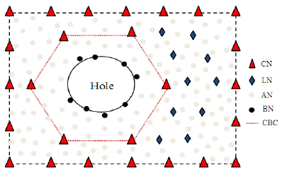
2.3.4 Landmark Node (LN)
These are the nodes within the network required for constructing a Virtual Hexagonal Landmark (VHL). Even if the network is of irregular shape, the LNs are deployed in hexagonal fashion which can be found in figure 4.
2.3.5 Boundary Node (BN)
These nodes tightly encircle the holes to form the actual boundary and is shown in figure 2.
2.3.6 Course Boundary Cycle (CBC)
The rough boundaries created by connecting the CNs is called Course Boundary Cycle. They are used for identifying each hole present in the sensing field and are found in figure 4.
2.3.7 Boundary Critical Point (BCP)
These are the intersection points between a particular node S with its sensing neighbors which cannot be covered by any of the other k nodes(where k is coverage degree). BCPs are shown in figure 5.
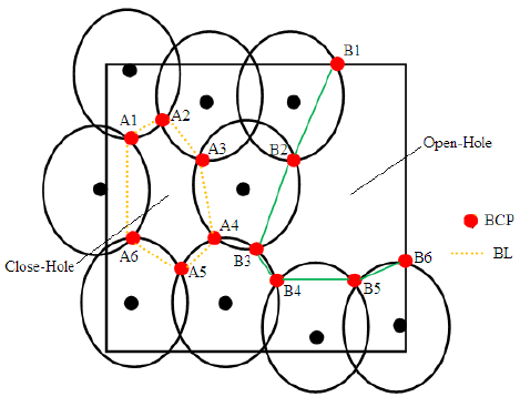
2.3.8 Boundary Line (BL)
The continuous BCPs while connected, forms the boundary line and are shown in figure 5.
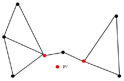
2.3.11 Pinch Vertex (PV)
A BN in a Delaunay Triangle is a pinch vertex, if it is a part of two or more distinct boundaries where two boundaries are called distinct if they have no mutual edge. Two PVs are shown in figure 6.
2.3.12 Delaunay Triangle (DT)
Let us assume a finite point set S in such a way that there is no point from S in its interior which means that the circumcircle of every triangle is empty. Therefore, the triangulation of the point set is called the Delaunay triangulation.
A triangulation of a finite point set S is called a Delaunay triangulation, if the circumcircle of every triangle is empty, i.e., there is no point from S in its interior. Figure 7 shows a DT.

2.3.13 Empty Circle Property (EC Property)
EC property is very useful for identification of DT. In this property, the unique circumcircle that passes through the three vertices of the triangle is called the empty circle of that triangle. It is shown in figure 8.

Here A(x, y) is the centre of the circumcircle whose coordinates are required to be calculated based on the position of the sensor nodes A1,A2 and A3. If A1(x1, y1), A2(x2, y2) and A3(x3, y3) are the 3 points (sensors) in the triangle whose coordinates are known, then using computational geometry, A(x, y) can easily be identified.
2.3.14 Stuck Node (SN)
A node p is called a stuck node if there exists a location q which is outside the transmission range but inside the sensing range in such a way that none of the 1-hop neighbors of p is closer to q than p itself. Figure 9 from [11] shows such a stuck node.

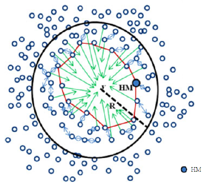
2.3.15 Hole Manager (HM)
At the end of hole-discovery(HD) process, the node having smallest Hole-ID is termed as Hole Manager. It removes its HD packet and announces the hole-healing. A HM can also be the node with the largest residual energy among all the boundary nodes. Figure 10 from [36] shows the HM node.
2.3.16 Inscribed Empty Circle (IEC)
An IEC is concentric with its corresponding empty circles and its radius is the difference between the radius of empty circle and sensing radius. In figure 11, 1 and 2 are the two IECs.

3 Algorithms for Boundary Detection
In this section, an elaborate discussion is done on the various algorithms available for coverage-hole & boundary detection.
3.1 Classification
Boundary detection algorithms are basically of three types- Topology based, Computational Geometry based and Statistical approach based. A details description of each category is provided in the following portions of this paper:
3.1.1 Topology based approach
This approach is based on topological properties like connectivity information to identify the boundary nodes. They do not need any extra location identification device such as GPS and hence cost is minimized. But they have to collect the neighboring nodes information and therefore high control packet overhead may occur. Still they have a moderate accuracy in boundary node detection w.r.t. statistical methods.
3.1.2 Covered Point (CP)
Let us assume a set of nodes Si, with sensing radius as RS, being deployed over a ROI. Then covered points are the points of intersections of Si with its neighboring nodes and are covered by any of the sensing neighbors of Si. Figure 12 shows such covered points.

In 2008, X. Liand D. K. Hunter proposed a distributed & coordinate free hole-recovery algorithm [28] where connectivity information is a prerequisite. At first, non-triangular coverage-hole is detected using the 3MeSH (Triangular Mesh Self-healing Hole Detection) algorithm. Based on the concepts of AN and RN and then using 3MeSH-DR (Triangular Mesh Self-healing Distributed Hole Recovery) algorithm, an accurate hole-boundary is detected by activating RNs adjacent to a hole and by checking whether two nodes are 2R units apart from each other or not.
In 2009, authors in [16] proposed a Distributed Boundary Recognition Algorithm (DBRA) based on node connectivity information to identify the boundary nodes surrounding the holes in the WSNs without using any location information. The four phases in DBRA are: (a) CNs selection - that approximately surrounds the holes and the border of the sensing field, (b) CBCs identification - that is used for identifying each obstacle present in the sensing field, (c) Detecting exact BNs - that senses the frontier nodes and attach them to filter the CBCs to be the final boundary and finally (d) Maintenance of BNs - is used to maintain the reliability of the BNs while boundary can be broken due to node failure. The exact BNs detection phase detects inner boundary that surrounds the holes and outer boundary that encloses the whole network. The BNs detection is based on energy usage which shows that the nodes in hole and network border consume more energy to discover the boundary.
In 2011, F. Yan et al. in [40] proposed a distributed algorithm with only connectivity information for non-triangular hole-detection. They have used Rips complex and Cech complex based on topological approach to discover coverage holes of type triangular and non-triangular. On the basis of neighboring node information, a method based on Hamilton cycle is used for hole-boundary detection. If any internal node has less than three neighbors or there is absence of any Hamiltonian cycle in its neighboring graph, then this node is considered to be on hole-boundary, otherwise, it is a non-hole boundary node. After boundary-node detection, the node itself is included to its neighbor graph to verify whether there exists Hamilton cycle in the newly formed graph or not.
I. M. Khan et al. in 2012 proposed a topological approach [22] for detection of boundary nodes based on connectivity information of every sensor node which are located at a given communication hop. The algorithm has three steps: (a) information collection - where every node identifies the list of its x-hop neighbors, (b) path construction - where the connectivity of the x-hop neighbors is reviewed to produce a communication path around each node and (c) path checking - where paths are further examined in order to infer the boundary and the inner nodes. If the communication path of a node's x-hop neighbors is broken, then the node is considered to be at the boundary and when the path is closed, the sensor is an inner node.
In 2014, B. Huang et al. proposed a distributed, local connectivity information based algorithm [17] for detecting both hole-boundary and network-boundary. For that the steps are: (a) identify suspected boundary - each node is roughly considered as boundary node or internal node based on a local variable which is initialized on its 2-hop neighbor node, (b) refine suspected boundary nodes - by exchanging the values of local variables between pairs of neighboring nodes, each suspected boundary node locally performs a heuristic operation to update the value of the variable and finally (c) searching tight boundary cycles - refined boundary nodes jointly search for boundary cycles based on their values of local variable and a set of tight boundary cycles corresponding to inner and outer boundaries are obtained.
S. Wan and Y. Zhang in 2017 proposed a Distributed, topology based approach [38] for hole-boundary detection. The nodes required to be self-aware of their co-ordinates. The steps are as following.
(a) identify i-Cones - these are a particular set of graphical structures where there are paths of length four which satisfy the empty i-Cones property. (b) identify central vertex - a unique central vertex, on any of the left or right sides of the path, is identified that is at a distance of two hops from the non-consecutive vertices. The side bearing this property encloses the face in its interior. (c) hole-boundary detection - for selecting the boundary edge, the following rules are applied: R1- marks the two central edges on the path which are incident to the central vertex as the hole-edges. R2 - is required in some obscure cases to ensure closure of paths. Under certain conditions, the rule un-marks a hole-edge in favor of the other to ensure connectivity.
The authors in [23] in the year 2018 proposed an algorithm which is distributed in nature and it was used to detect hole-boundary as well as network-boundary based on node connectivity information and estimated distance between nodes.
The steps are: (a) neighbor information -each node discovers its coverage neighbors and collects their information. (b) communication with neighbors - each node communicates with its neighbors to find whether its sensing range is fully covered by the sensing ranges of its neighbors or not. (c) boundary information - to complete the boundary information, the boundary nodes connect with each other and finally, (d) sub-graph formation - a boundary sub-graph amongst boundary nodes is constructed and classified either as an interior (hole-boundary) or an exterior boundary (network boundary).
The review works in topological approach of boundary detection is summarized in table 1.
Table 1 Summarization of topology based approach
| Ref | Algorithm | Features | Drawbacks | Future-Work | Simulator |
|---|---|---|---|---|---|
| [28] | 3MeSH | -coordinate free -detects large holes -less computational time |
Cant detect triangular holes |
Application on routing and jamming holes |
Matlab |
| [16] | DBRA | -connectivity based -less communication overhead |
Failure in multiple hole detection |
— | NS-2 |
| [40] | — | -triangular & non-triangular hole-detection -Hamilton cycle based hole-boundary detection |
Cant detect boundary holes |
Area estimation for varying sensing & communication radius |
Matlab |
| [22] | — | - X-hop neighbor matrix -works well with higher node degree |
Not scalable |
-will be applied on hybrid network -hole-avoidance |
GTSNetS |
| [17] | — | -hole & network boundary detection -energy efficient -boundary refinement |
Not scalable for high node density |
— | — |
| [38] | CHBA | -bypassing of hole -based on communication path |
-high communication overhead |
-practical implementation on real WSN testbed |
Matlab |
| [23] | hole and network boundary detection |
— | — | NS-2 |
3.1.3 Computational Geometry based Approach
This approach is based on node location information. They may collect the node location either by using GPS or to avoid higher cost, geometry based node localization methods may be used. Computational Geometry (CG) based approach is much accurate in boundary detection in comparison to topological and statistical approaches.
In 2009, J. Kanno et al. proposed a novel method [20] for detecting
number of coverage-holes along with their location in a coordinate-free sensor
network. In addition, they have detected the hole-boundary by processing
information embedded in a non-planar communication graph. This graph is
represented by a simplical complex and the first Betti number it is given as:
Z. Kang et al. in 2013 proposed a distributed algorithm [19] which is coordinate-free and connectivity-based. The algorithm is based on BCPs and can run on a single node by verifying the BCPs from neighbors. The connecting consecutive BCPs can form the BLs. The steps for finding BCPs are: (a) Node identification - a node in the network is identified and its neighbors are found and sorted clockwise, (b) Intersection point creation - A list of intersection points are created based on either node & its sorted sensing neighbors or node & the boundary of the monitoring region and finally (c) Intersection point verification - each intersection point is further verified whether it is a BCP or non-BCP and continue the process for all nodes.
For removing the redundancy in BCPs, it is assumed that any two neighboring
points such as bi and bj in the
list of BCPs will hold the relation as:
In 2014, P. Ghosh et al. proposed two novel distributed hole-detection algorithms [14] as DVHD (distance vector hole-determination) and GCHD (Gaussian curvature based hole-determination).
Using distributed Delaunay Triangulation, DVHD calculates the shortest distance path between any pair of nodes and utilizes path distance as metric for identifying the hole-boundaries. If the shortest path distance between two vertices is less than K (where K is a constant greater than no. of nodes), the two vertices are on the same boundary. If the shortest path distance between two vertices is greater than or equal to K, they are on different boundaries.
R. Jing et al. in the same year proposed a geometric-topologic hybrid method [18] for boundary detection meant for large-scale coverage holes in WSN based on minimum critical threshold constraint (BLW-MCT). The steps are: (a) Tree generation - directed shortest path tree is generated by the directed process of the network for the nodes, (b) Finding cut-vertex pair - from the directed shortest path tree, the minimum of the sum of distance between the cut node pair and least common ancestor is calculated and finally (c) boundary generation - from the cut node pair set and by comparing the minimum critical threshold with the product of the horizontal threshold and the vertical threshold of the cut node pair, the local large-scale coverage hole boundary is generated.
W. Li and W. Zhang in 2015 proposed a distributed algorithm [27] for hole-detection based on DT and empty circle property. The centers of the empty circles, containing the coverage-holes, are connected with lines in each pair of neighbor DT. If the line does not cross the common side of the two triangles or it intersects the common side whose length is greater than 2RS (where RS is the sensing radius), then the two empty circles, generated by the pair of neighbor DTs, incorporate in the same coverage hole. The empty circles can now be clustered to contain the same coverage hole into groups. Now, the boundary nodes of a certain coverage hole are the nodes that produce one group of empty circles.
In 2016, L. Zhao et al. proposed a distributed algorithm [44] for detecting both hole-boundary and network-boundary of the WSN. They have used the neighboring node location information based algorithm named, Distributed Sector Cover Scanning (DSCS), that is used to identify the nodes on hole-borders and the outer boundary of WSN. DSCS relies on the study that a node can have its own sensing area divided into dissimilar sectors by its neighbors and transforms the problem of identifying BNs into a decision that whether all the sensing sectors of a node are covered by the adjacent neighbors of the node or not. On the basis of 1-hop and 2-hop neighboring node information, the absolute angle of every node is calculated and arranged in the ascending order of their absolute angles to find the sectors. After broadcasting a 'hello' message by each node to its neighbour, the distance d1 is calculated. If d1 meets (k=1), then the neighbour is set as 1-hop. The 2-hop neighbour is calulated as:
In the same year, W. Li and Y. Wu in [26] proposed a distributed coverage-hole detection and tree-dissect based hole-healing algorithm (THH). In the tree, the IECs that are connected with only one extra IEC are called boundary IECs and are stored in a list according to their sizes. The largest IEC from the list is removed and is set as the source to construct a new sub-tree. The IECs that are neighboring to the source are removed from the list and added to the sub-tree and are set as the boundary IECs. If the radius of an IEC present in the list is smaller than that of its corresponding adjacent boundary IEC, then the IEC is removed from the list. The IEC is further added to the sub-tree and set as boundary IEC of the sub-tree until list is empty.
Again, R. Beghdad & A. Lamraoui in 2016 proposed Boundary Detection algorithm [4] based on Connected Independent Sets (BDCIS) and is divided in following three steps: (a) Collect connectivity information - by sending and receiving messages towards its neighbors, each node collects connectivity information and constructs its one-hop neighbors' graph only. (b) Create list of Independent Sets (iSs) - IS of cardinality a are established with the help of the minimum or maximum id in the graph Gi, which will be the first element of the IS1.
Then by removing all the neighbors of this node from Gi, another node having the minimum id among the remaining nodes is chosen and this process continues to build all other possible ISs. (c) Connection of ISs - for selecting the boundary nodes, the following rules are applied: Rule1- A node is internal if its 1-hop neighbors' graph has at least one IS of cardinality α or more and Rule2 - To connect each two nodes of the same IS there should exist a set of nodes that are not neighbors of another node in the set. Any node that does not satisfy both the rules is a boundary node. Otherwise, the node is selected to be an internal one.
In 2017, G. Zhang et al. proposed computational geometry based approach [42] for hole-detection and boundary identification in a hybrid sensor network. At first, the static sensors estimate the size of coverage-hole based on DT construction. Then the static sensors conduct the mobile sensors move to the optimal location to heal the coverage holes. Using computational geometry, bound of assisted sensor numbers is determined.
The review works in CG based approach of boundary detection is summarized in table 2.
Table 2 Summarization of CG based approach
| Ref | Algorithm | Features | Drawbacks | Future-Work | Simulator |
|---|---|---|---|---|---|
| [20] | Tri Collapse |
-coordinate free -applicable in all non-planar graphs -consider holes inside network |
Cant detect boundary holes |
-optimal hole patching -hole size estimation |
Matlab |
| [19] | -HDBCP -HPBCP |
-connectivity based - homogeneous network - Rc=2Rs -hole-patching -performs well for multiple holes |
-High computational complexity |
-real life application of the algorithm |
Matlab |
| [14] | -DVHD -GCHD |
-node location information based -DT -Incident angle |
High communication overhead |
-dynamic nodes -compliance to link failure |
Matlab |
| [18] | BLW -MCT |
-MCT constraints -large scale hole-detection -less computational overhead |
— | — | PLEX |
| [27] | ECA | -refines boundary -node clustering -hole and network boundaries detection |
Cannot detect boundary holes |
-hole healing with minimum cost |
Matlab |
| [44] | -DSCS -DW |
-node location based -hole & network boundaries detection |
-high communication overhead |
-hole healing -increasing network lifetime |
Matlab |
| [26] | THH | -tree-dissect based -hole-healing -optimal hole-patching |
False boundary detection |
-hole detection in directional sensor networks |
Matlab |
| [4] | BDCIS | -distributed -connected IS based |
-performs well in high node density |
-extension to low node density heterogeneous network |
Matlab |
| [42] | HCHA | -auxiliary node deployment strategy -hole-healing -hybrid network |
Cannot detect boundary holes |
-hole detection in directional sensor networks |
Matlab |
3.1.4 Statistical Approach
In this case, sensor nodes are assumed to be distributed uniformly in the ROI. There is no requirement of node location information in this case. Therefore, based on statistical property such as: probability of node distribution and under a specific network model, boundary nodes are identified. This approach has less accuracy in comparison to topology and CG based approaches.
M.R. Senouciet al. in 2014 proposed a distributed, localized algorithm [36], called HEAL (Holes Detection and Healing) that in the first phase, identify & discover the hole with hole-border detection and the second phase treats the hole healing by area determination and node relocation. For boundary detection the following steps are used: (a) SN detection - each node in the network uses TENT rule to detect whether they are SNs or not. The SN bi extracts the locations of the boundary nodes as: [b0, b1, …., bN].
Then it finds two nodes bn and
bm with highest distance as:
In 2016, L. Aliouane & M. Benchaiba proposed an algorithm [1] based on neighbor node's location information for hole-boundary detection and identification of hole. For boundary detection the required steps are: (a) Sorting neighboring nodes - each node detects its neighboring nodes and sort them in a list NSort(i). (b) Finding adjacent node - two nodes Sa and Sb are said to be adjacent node to Sc if the two nodes are sensing neighbors of Sc and there is no other neighbor of Sc between Sa and Sb and finally (c) Detecting boundary - this phase says that, if a node Sa checks if every two adjacent neighbors Sb and Sc are also neighbors of each other and if this is true for all its neighbors, the node Sa is not boundary. Whereas, if at least two adjacent neighbors of Sa are not neighbors, in this case, the node Sa is boundary node of a coverage hole.
Again in 2016, the authors in [25] proposed a coverage hole detection (DCHD) algorithm which is distributed in nature. The algorithm is used to detect the bounded or non-bounded coverage holes in a WSN. The set of BNs enclosing the coverage-hole are required to be identified before the hole-detection. The algorithm considers several points such as: location information of the nodes, sensing coverage overlap and the circumference of the non-overlapping region of the sensors.
The review works in statistical approach of boundary detection is summarized in table 3.
Table 3 Summarization of Statistical approach
| Ref | Algorithm | Features | Drawbacks | Future-Work | Simulator |
|---|---|---|---|---|---|
| [36] | HEAL | -node relocation -deterministic deployment -hole-area determination |
Cannot detect boundary holes |
-on demand hole detection -holes with obstacles |
NS-2 |
| [1] | — | -coordinate based -Rc >= 2Rs |
-local hole detection -high communication overhead |
Hole-recovery | NS-2 |
| [25] | DCHD | -critical intersection point based -hole clustering - hole and network boundary detection |
-high computational overhead |
-hole detection in irregular ROI -hole-recovery |
NS-2 |
4 Performance Analysis & Summarization
In this section, based on different categories of boundary detection algorithms, performance analysis was carried out. It gives a clear idea about the various measurement techniques used by different authors to evaluate the performance of their respective algorithms. Also we have tried to identify few research issues in each category of algorithm.
4.1 Performance Analysis - Topology based
In [28] evaluation is done based on mean no. of recoverable holes in different node density. For medium node density, no. of recoverable holes is larger and for higher node density, average no. of unrecoverable holes is smallest. Also it compares hole-recovery iterations with and without further hole-detection. Detection of unrecoverable hole converges after 7th iteration. In [16] evaluation is done based on accuracy ratio, control packet overhead & simulation time. Also the effects of node degree & number of holes were analyzed. Even if node degree is higher, algorithm shows high accuracy ratio.
For higher number of holes, control packet overhead is less and the simulation time increases a little. In [40] evaluation is done based on percentage of area of triangular holes for a given intensity. With increasing intensity percentage of area of triangular holes decreases. Also with higher intensity, error probability of hole-detection increases. In [22] evaluation is done on based on percentage of true boundary node detection w.r.t. given degree of node.
Performance of 1-hop approach decreases with increasing node density and 2-hop & 3-hop approach gives better performance. Again 2-hop & 3-hop approaches consume more energy than 1-hop approach but 1-hop approach is unable to produce accurate boundary-node detection. In [17] evaluation is done based on node density, distribution & wireless channel model. Higher node density increases the chance of forming closed path encircling interior nodes and therefore decreases the chance of wrongly identifying internal nodes as suspected boundary nodes. For low node degree, distribution of node is satisfactory by reducing formation of cluster & small holes. In [38] evaluation parameters are runtime and message count per node.
Proposed algorithm shows run-time decreases with increasing no. of holes for a network when node density is fixed in the ROI. Again, message count per node remains almost similar with increasing no. of holes in the network. In [23] evaluation parameters are no. of boundary nodes, communication overhead & energy consumption. With increasing node density, no. of holes decreases so no. of boundary nodes also decreases. With increasing node degree, no. of message passing in between each neighboring nodes increases which in turn increases the communication overhead. And finally, with increasing network density with fixed average degree decreases the energy consumption.
Summary: Having a moderate accuracy of boundary detection, connectivity information is the key to this approach. Sudden topology changes can result high communication overhead & failure in multiple hole-detection. Here the evaluation parameters are: boundary-detection time, energy consumption, accuracy ratio and control packet overhead based on the effects of node density, wireless channel model, message count per node, average node degree etc. Figure 13 shows the comparison of boundary detection accuracy in between [16,22] where the detection accuracy of [16] is higher with lower node degree.

4.2 Performance Analysis - CG based
In [20], evaluation parameters are: run-time and accuracy of hole-detection and the effects of no. of nodes, no. of holes and size of holes are analyzed. If no. of nodes increases, run-time increases exponentially and if no. of holes increases, runtime increases very slowly. If size of hole, i.e no. of boundary nodes increases, run-time decreases.
In [19], evaluation is done based on coverage analysis. For increasing node density, the recovery degree by patching nodes also improves.
The evaluation is done in [14] based on run-time with increasing no. of holes. If the no. of holes increases, no. of boundary nodes also increases hence, average no. of neighbors per node decreases which reduces run-time slightly. Also, no. of message exchanges per node in the network increases with increasing no. of nodes, whereas, the average no. of message remains almost same with the increasing no. of holes.
In [18], evaluation parameters are: size of packets, boundary detection time and boundary discovery numbers. The size of packets decreases with increasing node density because the increasing nodes decreases hole-number & thus size of packets also decreases. Boundary detection time decreases with increasing nodes because increasing nodes mean less probability of holes & hence detection of boundary nodes also decreases. Also, boundary discovery no. decreases with increasing node density.
The evaluation parameters in [27] are ROI size, average no. of detected holes and no. of boundary nodes. It can be seen that with increasing ROI, course boundary nodes and refined boundary nodes increase. With fixed node density, if ROI size increases, sensing range decreases and chances of hole-occurrence also increases which results course boundary nodes and refined boundary nodes increment. Since both triangular and non-triangular holes can be detected, hence this algorithm has higher average no. of detected holes. Again, no. of boundary nodes is less since the algorithm can refine boundary nodes.
In [44], evaluation parameters are boundary detection rate, runtime and energy efficiency w.r.t size of ROI and length of communication radius. The algorithm shows higher boundary detection rate and lower false detection rate with increasing network size. No. of boundary nodes increases with increasing ROI and it decreases with the increasing communication radius.
If same no. of nodes is deployed in varying ROIs, node density decreases that reduces each node's neighbors and hence BNs' occurrence probability increases. Again, with increasing communication radius, node density increases which decreases BNs' occurrence probability. Again, with higher node density and communication radius, energy consumption increases.
The proposed algorithm in [26] gives better coverage with additional no. of node deployment.
The evaluation parameters in [4] are accuracy, energy consumption and communication overhead with varying node density. Proposed algorithm accurately detects boundary nodes with varying average node degree. For increasing node density, each node broadcasts a message that will be received by all its neighbors and hence energy consumption in message broadcasting increases. Again, the communication overhead also increases with increasing node degree.
In [42], evaluation parameter is the coverage ratio. Authors claimed better coverage ratio with increasing static nodes.
Summary: This is the most popular approach among all the three approaches due to their accuracy in boundary detection. As node deployment is random, hence prior node location information is a must in CG based approach. Although, this method is very precise in detecting both hole & network boundary but sometimes the drawback is to detect hybrid-holes formed in combination with a few node along with the network boundary. CG based approaches mostly use Matlab as a simulator due to high-end mathematical functions.
Here the evaluation parameters are: boundary-detection time, energy efficiency, detection accuracy and communication overhead based on the effects of no. of nodes, no. of holes, size of holes, no. of message exchanges, average node degree etc. Figure 14 shows the comparison of boundary detection accuracy between [4,44] where [4] shows better accuracy with lower node degree.

Again, figure 15 shows the comparison between [18] and [20] w.r.t. boundary detection time where [18] requires less time for boundary detection.

4.3 Performance Analysis - Statistical based
Authors in [36] did the performance evaluation based on the no. of holes and varying size of holes. With increasing hole-radius, no. of node movement increases and the nodes closest to hole moves longer distance w.r.t. the border nodes. This is because, with increasing hole-radius, hole-area increases and to repair it, node density should be higher. Again with the increasing node density, the algorithm performance improves w.r.t. travelled distance, no. of movements and rate of improvements in network coverage.
In [1], evaluation parameters are detection accuracy and total energy consumption. For higher node density, the algorithm consumes less energy to detect holes due to local hole-detection. Authors also claimed the hole-detection accuracy is better and almost all boundary nodes can be detected since more nodes participate in boundary node detection process.
Again in [25] evaluation parameters are control packet overhead and power consumption to detect the holes and time to detect the holes. Average hole-detection time and control packet overhead increases with higher node density. Again, energy consumption increases with increasing number of holes.
Summary: Since, in this approach node distribution is uniform, hence node location information is not essential. While the performance measurement techniques can be no. & size of holes, energy consumption and control packet overheads, this approach has the cons of high communication & computational overhead.
Due to their less accuracy, statistical approaches are not as much in use as compared to the other two approaches. The comparison between the average energy consumption of [1] and [25] is shown in figure 16.

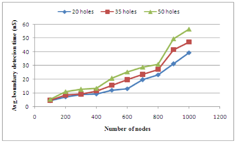
Again, figure 17 shows the average boundary detection time with respect to different numbers of holes from [25]. From figure 17, it is clear that with increasing number of coverage-holes in the system,, boundary detection time also increases.
5 Research Queries
As per the main three approaches of boundary detection, research has been carried out since long to provide solutions to various research problems.
However, during the review of the different papers in this field we could formulate a few research queries which need to be solved.
5.1 Self-Organizing Coverage Control
In a WSN, the main reason behind coverage-hole occurrence is the failure of the sensor nodes which can be amplified due to increasing distance between nodes or energy consumption. Therefore, if a large quantity of node-failure transpires, then there must be some techniques which can organize the rest of the nodes very promptly for coverage control. This is what is called self-organizing coverage control and further research is required for this automated coverage control.
5.2 Hole-Clustering
Due to random deployment of the sensors in a WSN, some nodes form holes inside the network and some other can form holes along with the network boundary. Therefore, hole-clustering is the technique of identifying whether the holes are present inside the network or at the network boundary.
The reason behind hole-clustering is energy preservation as energy scarcity in WSN is a big issue. Also clustering of holes can reducing data redundancy in the network by load balancing in the WSN.
5.3 Hole-Area Estimation
To achieve an autonomous & self-organizing coverage control, hole-area [8] is required to be calculated since it estimates the uncovered area in the ROI. Due to random deployment of sensors, they even overlap which may cause unnecessary dense arrangement in the ROI. Therefore, based on hole-area estimation, accurate no. of sensors can be deployed to fill up the coverage-hole.
5.4 Optimal Hole-Patching
After the hole-area estimation, the boundary nodes surrounding the holes and the dead-nodes which are responsible for the creation of holes are detected. The idea behind hole-patching is to increase the network coverage based on network topology and connectivity. In this phase, the dead-nodes are patched or replaced with the ANs so that the SNs could be recovered.
Meanwhile, optimal hole-patching deploys minimum possible sensors to fill up the holes which may reduce the hole-recovery overhead. Therefore, further research can be done on these techniques to maintain the network connectivity by deploying new nodes so that the average packet delivery time can be reduced.
6 Conclusion
Hole-boundary is able to cluster the whole network based on the presence of coverage-hole, hence, coverage-hole boundary detection is one salient research topic in the field of WSN. In this paper, we have categorized various boundary detection algorithms and also made a performance analysis of each of them. Based on that analysis, we also have raised a few research queries which may be helpful for future direction of work in this field.
The research queries include the automated coverage control which is directly associated with the QoS of WSNs. Hole-clustering and hole-area estimation is also tightly bound with coverage and connectivity issues. Finally, optimal hole-patching is very essential to estimate the minimum number of nodes required to fill up the coverage-holes such that energy efficiency is maximum.

