


 text new page (beta)
 English (pdf)
 Article in xml format
 Article references
 Send this article by e-mail
 Cited by SciELO
  Similars in
SciELO
Similars in
SciELO 
 Permalink
1 Introduction
Automatic image annotation (AIA) consists of assigning keywords to images to describe their visual content. AIA has been traditionally approached as a supervised learning task, where, given a dataset formed by image-label pairs, a function (i.e., a classifier) mapping images to labels are learned. In this scenario, the classes for the classifier correspond to labels that can be used to annotate images (like "animal", "transport", "fruit", for example). The performance of supervised AIA methods is acceptable, mainly when the number of labels is small. In principle, with this approach, it is possible to assign whichever label to images. Although in practice, this process is constrained to assign a limited number of them, that is, only those concepts present in the training dataset, e.g., see ImageNet [38].
If we increase the number of considered labels, the complexity of the associated model increases considerably. Consequently, datasets for AIA have traditionally considered only a few concepts to describe images (e.g., Caltech 256 [17], PASCAL [9] datasets), which makes the classification quite specific and limits the diversity in the label assignation process.
To alleviate the foregoing limitations of supervised AIA methods, unsupervised formulations have been proposed as well [31]. These methods aim to discovery text-image associations by mining large collections of multimodal documents. Unsupervised AIA techniques relax the limitation of reduced annotation vocabulary. However, its performance is commonly lower than that of supervised techniques.
Supervised and unsupervised AIA methods cannot offer both vocabulary diversity-scalability and high performance. Alternatively, the AIA problem can be approached as a text-image matching task, and this can be formulated as a binary classification problem [32]. In a nutshell, image and textual descriptors are concatenated to form a heterogeneous input space. The classes for samples are given by the relevance of a word to the image, see Figure 1.

Since this formulation is based on supervised learning, it inherits the high performance of supervised AIA methods.
Likewise, since in principle, any text-image can be represented in such input space, any word could be considered for describing an image. Figure 2 illustrates the considered scenario.

Fig. 2 A general framework used for generating positive/negative instances of the approached problem. The representations of images and words are concatenated to produce the instances of the binary classification task
To study the feasibility of the suggested approach, we organized an academic competition on text-image matching. Academic challenges have been successfully used in many domains as a mechanism to advance state of the art (e.g., ImageNet1, ChaLearn Looking at People challenges2), allowing the community of researchers to propose competitive solutions to specific tasks. With this purpose in mind, we generated a challenging dataset for text-image matching and asked participants to develop solutions for the problem.
In addition to data, we provided an evaluation protocol and prizes to encourage participants. The challenge was run in the CodaLab platform and attracted more than 40 participants, and results suggest that the proposed formulation is a promising solution to the AIA problem. This paper describes in detail the challenge design, summarizes its main results, and performs a detailed analysis of the best three methods developed by the participants.
This paper is an extended version of [32], where a summary of results was reported. This paper goes several steps forward, by providing a detailed description of the design of the challenge, a complete analysis of results, and an in-depth description and analysis of the top three teams that participated in the challenge.
2 Related Work
Generating training data for supervised image classification methods is generally performed manually, in the best cases, by using crowd services (e.g., Mechanical Turk [36]). Although the quality of this sort of methods is commonly acceptable, manually generating labels can be an expensive and laborious endeavor. Besides, datasets generated in this way only cover a reduced number of labels (concepts) and are subject to bias/noise.
Notwithstanding the above, some methods have been proposed with the aim to label images with large annotation vocabularies. For instance, in [4], a fully-automated system for learning everything about any concept was presented. The idea behind this method consists of processing books and images on the Web intertwining the data collection through their variances. The system was able to model 760 concepts using approximately 233M images3, although somewhat scalable, 760 concepts are far away from being 'everything.'
In the same path, several semi-supervised approaches have tried to alleviate the problem of learning any concept using unlabeled data (e.g., see [34,3]). These methods assume that unlabeled data can be used to extract knowledge to improve the one found in small datasets. One way to incorporate unlabeled data is by using transfer learning. The purpose of transfer learning is to translate knowledge/information from a source domain to a target domain, often using a single feature space [2]. Different approaches for transfer learning have been proposed so far, from traditional machine learning approaches, e.g., see [35,42,2,30,45], to the most recent through the use of deep learning, where pre-trained models obtained by a convolutional neural network can be exploited for feature extraction [37], or fine-tuning its architecture [43].
On the other hand, unsupervised AIA methods rely on text mining methods that process collections of weakly labeled images (e.g., web pages and the images they contain) to assign free-vocabulary labels to images, e.g., see [19,26,31]. The assumption is that text that accompanies images is at some level related to the visual content; and therefore, this can be employed in the labeling process. In this regard, the extracted vocabulary by unsupervised AIA methods can be larger than the used by supervised AIA ones; however, its main limitation is the inherent noise in weakly labeled images.
In this work, we rely on a simple transfer learning methodology to obtain a representation for images to be used in a novel AIA formulation based on text-image matching. The proposed approach cast the AIA problem as one of binary classification. When compared to supervised AIA methods, the proposed approach maintains the high performance of this sort of models. While, when compared to unsupervised AIA techniques, the proposed approach can work with large annotation vocabularies.
3 Text-Image Matching Challenge
The RICATIM challenge was run in the CodaLab4 platform and had a duration of about 45 days. The task approached by participants was that of determining the relevance of words to describe the content of images. More specifically, participants had to develop binary classification methods for determining the relevance (positive class) or not (negative class) of words to describe the visual content of images. Vectorial descriptors were extracted from each image and from the word separately (see details below). Both representations were concatenated, giving rise to a heterogeneous text-image representation. A challenging dataset was generated in this way, assigning classes to each instance according to the relevance of the word to describe the visual content of images (see Figure 1).
The dataset was split into training (development), validation, and test partitions.
Labeled training data and unlabeled validation data were made available at the beginning of the challenge. During the challenge, participants could submit predictions for the validation set via the CodaLab platform and receive immediate feedback on their validation performance via the leaderboard. At the end of the development phase, unlabeled test data were released, and participants had a few days for submitting predictions for these data. Performance on the test set was used to determine the winners of the challenge.
Two baseline methods were implemented; the first one was simple enough to give the participants a wide margin for improvement. This baseline was a machine learning approach using a support vector machine (SVM) with LIBLINEAR [10] without performing any preprocessing in the data. The second point of comparison was defined using the random forest implementation from the CLOP5 toolbox.
This challenge was organized and sponsored by RedlCA6: Red Temática CONACyT en Inteligencia Computacional Aplicada, and it was expected to be the first of a series of periodic challenges organized by this academic network. To be eligible for prizes, the winners had to release their code publicly and submit fact sheets describing their methods. The source code of every participant was verified and replicated before announcing the winners.
The timeline for the challenge was as follows:
— July 3, 2017: Beginning of the challenge, release of development and validation data.
— August 14, 2017: Release of test data and validation ground truth labels.
— August 16, 2017: Submission deadline for prediction in the test set. Release of worksheet template.
— August 18, 2017: Submission deadline for code and fact sheets.
— August 19 - August 23, 2017: Verification phase (code and fact sheets).
— August 24, 2017: Winners notification.
— September 4 - September 8, 2017: Presentation of results at ENIAC-SNAIC and award winners.
4 The RICATIM Dataset
For the organization of the challenge, we developed a novel dataset on text-image matching called RICATIM7. An instance in this dataset consists of a concatenation of a visual and a textual representation (see Figure 2). For representing images, we used CNN-based features extracted by using a pre-trained deep neural network: each image was preprocessed and passed through a pre-trained 16-layer CNN-model [39], the penultimate layer activations were used as the visual representation for images (a vector of 4096 elements).
On the other hand, keywords were represented by their word2vec representation [29] (200-dimensional vectors were used). Word2vec representations were obtained by using Wikipedia as training collection. After the generation of individual image and text representations, both input spaces were concatenated to form the input space for the text-image matching challenge, consisting of 4,096 attributes from each image and 200 attributes from the text, all associated with a binary class.
Below we describe the way we generated the labels for instances of this mixed input space. For the creation of the RICATIM dataset, we randomly selected a set of 3,300 images from the IAPR TC-12 dataset [18,8]. The IAPR TC-12 collection consists of 20,000 real-world images. Every image has a manually generated caption/description, see (f) in Figure 3. The segmented and annotated IAPR TC-12 (SAIAPR TC-12) benchmark [8] is an extended version where images were manually segmented and annotated at the region level (i.e., see (e) in Figure 3) with about 250 keywords (hierarchically organized). We used labels information from both the IAPR TC12 dataset and its extended version for preparing the RICATIM dataset.

Fig. 3 Sample of images from [18,8]: (a)-(d) images taken by tourism travel agencies; (e) segmented images; and (f) image accompanied by its metadata
To generate the labels of instances for the dataset, the initial 3,300 images dataset was divided into three subsets: X, Y and Z containing the same number of images. Each subset was processed differently to generate labels. The aim was to produce more diversity into the created instances. The adopted strategies are depicted in Figure 4, and are described as follows:
— Region-level labels. For the X subset, we used the labels assigned to images according to the considered dataset. For a given image i ∈ X, the generation of positive instances (relevant text-image pairs) was straightforward: manually assigned labels to image i were considered as relevant. The labels for negative instances (nonrelevant text-image pairs) were produced by randomly taking labels from the semantically-farthest keywords to the manually assigned labels. The semantic distance was estimated by the distances among the word2vec representations of labels.
— Annotated captions. For the Y subset, we used descriptions to generate classes, see (f) in Figure 3. First, descriptions were indexed with a bag-of-words (BoW) model; then, a TF-IDF weighting scheme was applied. For generating positive instances, given an image i ∈ Y we considered as relevant labels those words from the caption with higher TF-IDF value. As the vocabulary extracted from the captions is large, i.e., 7,708 different terms, the terms used as negative were not taken from the last positions. Instead, using the word2vec representation corresponding to whole extracted vocabulary, a matrix of cosine distances among these vectors was calculated. Thus, empirically a distance range was chosen to take terms to be used as negative, i.e., the negative label for a given positive label was randomly taken from the nearest 200-400 labels to the positive one (we found related, but irrelevant, words in this range).
— Unsupervised Automatic Image Annotation. In this case, we used a UAIA method proposed in [31] to generate relevant and irrelevant text-image pairs for set Z. We integrate this strategy into the creation of the dataset because we focus on a hybrid approach to AIA. Note that AIA methods commonly use a cleaner ground truth but less diverse than those assigned by considering a free-vocabulary.

Fig. 4 Strategies adopted for representing labels assigned to images in the instance generation process
In each of the subsets/labeling-strategies, a negative instance was generated per each positive one, taking special care that labels used as negative were different from the positives. A different number of instances was created from each image, depending on the number of words assigned to it in the reference collection. In the case of the X subset (i.e., region level approach) an average of eight labels was used. The other two strategies tend to generate a varied number of positive and negative instances for each image, in a range between three and six labels. In the end, both sets had an average of 10 annotations per image, among positive and negative labels.
From the three strategies used in the methodology, a total of 31,128 instances were generated. Then, we selected 30,000 random instances from the different subsets to create the following disjoint subsets:
— Training data (labeled data, can be used to train and develop models). This partition is formed by 20,000 instances, where 40% are positive instances, and 60% are negative instances.
— Validation data (unlabeled data, participants can make predictions during phase 1 to get immediate feedback in the leaderboard). This partition is composed of 5,000 instances, 60% positive and 40% negative instances.
— Test dataset (used to determine the winners). This partition is composed of 5,000 instances, but this time 50% are positive instances, and 50% are negative instances.
Finally, instances in each partition were shuffled with the aim to avoid learning the construction pattern. Additionally, we also provided raw images and the actual words used to generate instance in case participants wanted to take advantage of such information.
5 Summary of Results
In this section, we summarize the results obtained in the challenge, while the next section presents the detailed results with the descriptions of the top ranked methods.
The competition attracted 43 participants that made more than 220 submissions to the leader-board. Figure 5 shows the number of submissions per participant. It can be observed that several participants contributed with a large number of submissions.

Figure 6 shows the validation performance of submissions vs. time. The baselines (marked with red circles) were outperformed since the very beginning of the challenge. Still, at the end of the challenge, some of the participants overfitted the validation data (accessible from the leaderboard).

Fig. 6 Performance of submissions vs. time (the red circles indicate the performance of the baselines)
Table 1 summarizes the results of the top-ranked participants in the competition (the information between brackets indicates the team to which different participants belong to). The top four participants were successful in outperforming the baselines and achieving recognition rates close to 0.9. In the following section, we describe in detail these methods, and later, we analyze in depth their performances.
Table 1 Performance measures (in %) for the all techniques
| System (TEAM) | Accuracy | F1 | ||
|---|---|---|---|---|
| dev. | test | dev. | test | |
| Organizing team | ||||
| Baseline 1 | 0.644 | 0.639 | 0.69 | 0.64 |
| baseline 2 | 0.760 | 0.818 | 0.76 | 0.79 |
| I3GO+ team | ||||
| job80 (T1) | 0.831 | 0.838 | 0.85 | 0.84 |
| ClaudiaSanchez (T1) | 0.816 | 0.823 | 0.84 | 0.82 |
| mgraffg (T1) | 0.813 | 0.824 | 0.84 | 0.82 |
| dmocteo (T1) | 0.684 | 0.833 | 0.71 | 0.83 |
| sadit (T1) | 0.797 | 0.844 | 0.82 | 0.84 |
| MIGUE, TAVO & ANDRES team | ||||
| migue (T2) | 0.811 | 0.830 | 0.83 | 0.82 |
| octavioloyola (T2) | 0.807 | 0.834 | 0.83 | 0.83 |
| andres (T2) | 0.801 | 0.824 | 0.82 | 0.82 |
| Voltaire Project team | ||||
| Phoenix (T3) | 0.823 | 0.828 | 0.85 | 0.83 |
| Argenis team | ||||
| argenis (T4) | 0.758 | 0.780 | 0.78 | 0.78 |
| Individual participants | ||||
| Naman | 0.656 | — | 0.72 | — |
| Miguelgarcia | 0.600 | — | 0.75 | — |
| Barb | 0.479 | — | 0.48 | — |
| Victor | 0.499 | — | 0.55 | — |
6 Top-Ranked Methods
In this section, we present the top three ranked methods in the final phase of the challenge. For each method, an analysis of its performance is included. The top-3 ranked methods were considered for the study. Their overall performance is shown in Table 1. For completion, Table 2 shows the performance of the considered teams on the different subsets of data that were used to generate the labels (see Section 4). The reported score corresponds to the micro-average accuracy, where each subset is considered individually.
Table 2 Performance accuracy (in %) according to the label source creation
| Team (methods under their best settings) |
micro acc. (regions) |
micro acc. (captions) |
micro acc. (UAIA) |
|---|---|---|---|
| method proposed by I3GO+ | 0.925 | 0.922 | 0.691 |
| method proposed by MIGUE, TAVO & ANDRES | 0.913 | 0.916 | 0.677 |
| method proposed by Phoenix | 0.911 | 0.908 | 0.670 |
In the third column, we can see that the most challenging subset for classification was the subset generated from the labels provided by the UAIA method, while the proposed solution methods achieved similar performances in the other two columns (1 and 2). These results suggest that the labels provided by the UAIA method can be noisy or to refer to concepts that are difficult to correlate with visual information. In the following, we provide more details on the solutions from the top 3 ranked participants.
The organized challenge was a success in terms of participation and performance achieved by the solutions in the text-image matching approach to AIA. To gain further insights into the nature of methods and their performance, in the rest of this paper, we describe the top-ranked methodologies and perform an extensive study comparing their performance.
6.1 I3GO+ (First Place)
We start describing the solution that won the RICATIM challenge. The proposal consists of generating a new low dimensional space by approximating the k centers problem using the Farthest First Traversal algorithm (FF-traversal), along with a kernel function. The new representation feeds a kNN classifier. By using this approach, the dimension is reduced, and the final performance is improved. Below we describe each of the steps involved in this solution, a graphical description of this method is provided in Figure 7.

6.1.1 The k-Centers Problem
Finding a solution for k-centers is equivalent to the generate є-nets problem ([40]). From this point of view, k-center is an optimization problem, where the objective is to find a set of centers C={ci,c2, … ,ck} of cardinality k = |C|, and where all elements xi ∈ X are at most distance є from its nearest center in C. The precise value of є is optimized for a particular value of k, and conversely, k can also be optimized for some є.
6.1.2 Farthest First Traversal
The Farthest First Traversal (FF-traversal) algorithm was proposed simultaneously in [15] and [20]. The algorithm finds the best know approximation (in polynomial time) for the k-centers problem, i.e., at most two times the optimal solution. Finding any best approximation is NP-Hard (see [15,20,11]).
The algorithm of T.F. Gonzalez [15] calculates a set C, where all cj ∈ C are farthest among them. So, for each x ∈ X, the distance to the nearest centers is kept in C, the distance for each xi is updated each time that a new cj is added to C. In order to ease the algorithm definition let use define dmin(x) as the distance between x and its nearest center in C, then dmin(x) = min{d(x, c) | c ∈ C}. Algorithm 1 specifies the FF-traversal:

Given some starting element for C, the farthest object in X \ C to all objects in C is located in each iteration, and then it is added to C. This order resembles a farthest-first walk or traversal over X, and this fact gives the name to the algorithm. Let r be the distance used to choose the new center; it follows that at each FF-traversal iteration, a Delaunay set is built; the following properties are preserved:
— Any pair of objects xp, xq ∈ X are at distance at least r from each other
— Any elements xq ∈ X are at most distance r from one of the cj ∈ C
So, the FF-traversal algorithm finds k elements that minimize the maximum distance between the elements x ∈ X to some c among the available centers C. Figure 8a shows the Delaunay set generated from 5 normal distributions with four items each one. Each ball radius is the optimal r found at iteration 5. Moreover, Figure 8b illustrates the order of how FF-traversal selected the five centers in C.

6.1.3 Kernelized k-Centers
The proposed solution is based on the hypothesis that chosen centers are good
enough to represent the complete database variation; hence selected centers are
used to create a lower dimensional space. The new feature space is created by
mapping all the objects in X to the new space
X’, and X’ is used as training dataset for
a k-nn classifier. The new features for each
xi are generated using a function
Φ(x, C) over each
xi and the elements in C; i.e.
For the presented experiments when using RBFs, the parameter σ is set to the є found at the last iteration of the FF-traversal algorithm. Algorithm 2 describes the feature generation algorithm:
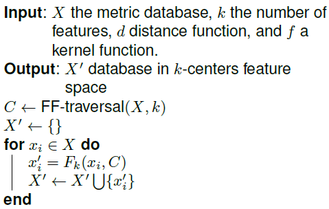
This approach is named FF-traversal for Feature Condensation (FFTFC) and the generated feature space as k-Centers Features. The resulting process is composed of two main stages:
6.1.4 Experimental Setup
The authors tried several related approaches. Firstly, this proposal used the FFTFC over the official image vectors and the plain word2vec features. To control the significance of each kind of feature, the authors introduced a weighted metric dW, defined in Equation 2:
where W ∈ [0,1]. By using Equation 2 the weight W is used to adjust the contribution of each feature portion (i.e., image and text). The kernel function may use the set of centers C, or the set of centroids Ĉ. Each centroid ĉ∈Ĉ is computed using c, where each component of ĉ is computed as the average of that component over all items having c as its nearest center c∈C.
Also, a set of additional features for text labels were produced with μTC library (see [41]). Feature vectors obtained with μTC are sparse vectors of dimension m = 3951, these features were concatenated to the image data to get 8047-dimensional vectors. A new set of k-Centers features were created using this new representation. A standard PCA dimensionality reduction and the nonlinear Kernel PCA (KPCA) were compared with FFTFC. All results in this approach were computed using an RBF kernel, for both KPCA and FFTFC.
The selection of the classifier and its parameters were performed using a cross-validation split of 70% for the training set and 30% for the validation set. The resulting features were used to fit a kNN (k=3) classifier. Table 3 shows the obtained results for the four evaluated metrics at the RICATIM Challenge. As can be seen, over the 70-30 split, the k-centers and KPCA outperforms PCA and exhibit similar scores. However, k-Centers features have lower dimensionality. For the sake of completeness, the scores using the original feature space are also shown at Table 3. The best result of each score is marked using boldface.
Table 3 Comparison of k-Centers and standard techniques to reduce the dimension
| Method/ Features |
Orig. dim. |
Red. dim. | Ref. | Dist. fun.(d) |
Acc. | Recall | PR | F1 |
|---|---|---|---|---|---|---|---|---|
| k-Centers/Img | 4296 | 264 | centers | L2 | 0.802 | 0.801 | 0.733 | 0.797 |
| k-Centers/Img | 4296 | 264 | centers | Cosine | 0.810 | 0.810 | 0.738 | 0.805 |
| Original | 4296 | — | — | — | 0.483 | 0.471 | 0.368 | 0.470 |
| PCA/Img | 4296 | 264 | — | — | 0.487 | 0.474 | 0.372 | 0.474 |
| PCA/Img | 4296 | 328 | — | — | 0.488 | 0.475 | 0.372 | 0.474 |
| PCA/Img | 4296 | 456 | — | — | 0.480 | 0.469 | 0.367 | 0.468 |
| KPCA/Img | 4296 | 264 | — | — | 0.808 | 0.811 | 0.730 | 0.804 |
| KPCA/Img | 4296 | 328 | — | — | 0.806 | 0.807 | 0.733 | 0.801 |
| KPCA/Img | 4296 | 456 | — | — | 0.811 | 0.812 | 0.740 | 0.806 |
| KPCA/Img | 4296 | 712 | — | — | 0.811 | 0.811 | 0.741 | 0.806 |
| k-Centers/Img + μ _TC | 8047 | 140 | centers | WCosine (W=0.96) | 0.821 | 0.817 | 0.764 | 0.815 |
6.1.5 Performance at Development Phase
During the development phase, an ensemble of three of the previous classifiers was tested. Results obtained are shown at Table 1, the top result for I3GO+ team are the results of an ensemble with a majority class for the three k-Centers features show at Table 3, while second and third rows at Table 1 are the resulting scores for EvoDAG based classifiers (see [16]) over k-Centers features. Table 4 shows the top three results for the proposed scheme. It is relevant to mention that the first one was the best score at the development phase.
6.2 An Approach based on Contrast Patterns (Second Place)
This section describes the proposal that obtained a second place in the RICATIM challenge. Additionally, this section shows the experimental results attained for each pattern-based approach using the original RICATIM database as well as the experimental results achieved but using a new RICATIM database representation, which was introduced by the I3GO+ team (see section 6.1).
6.2.1 Classification Based on Contrast Patterns
Over the past years, several classifiers have been proposed in the literature but nowadays obtaining a high accuracy is not the only desired characteristic for a classifier; experts in the application domain should understand the results associated to each class of the problem [44,25].
Contrast pattern-based classifiers are an essential family of both understandable and accurate classifiers. The main reasons are that contrast pattern-based classifiers provide patterns in a language that is easy for a human to understand, and they have demonstrated to be more accurate predictions than other popular classification models, such as decision trees, naive Bayes, nearest neighbor, bagging, boosting, and the support vector machine (SVM) [44,25].
A classifier based on contrast patterns uses a collection of contrast patterns to create a classifier that predicts a query object class [44].
A pattern is represented by a conjunction of relational statements, each with the form: [f # vj], where vj is a value in the domain of feature fi and # is a relational operator from the set {=, ≠, ≤, >} [28,25]. For example, [Height ∈ [1.9, 2.1]] ˄ [Weight ≤ 120] ˄ [Agility = "Excellent"]] I a pattern describing a collection of basketball players. Let p be a pattern and T be (often) a (training) dataset; then, the support of p (with respect to T) is a fraction resulting from dividing the number of objects in T described (covered) by p by the total number of objects in T. Now, a contrast pattern (CP) for a class c is a pattern whereby the support of CP for c is significantly higher than any support of CP for every class other than c[6,5,25].
Contrast pattern-based classifiers are used in various real-world applications, such as gene expression profiles [7], structural alerts for computational toxicology [33], gene transfer and microarray concordance analysis [27], characterization for leukemia subtypes [24], classification of spatial and image data [23], and heart disease prediction [21], in which they have reported effective classification results.
For building a contrast pattern-based classifier, there are three phases: mining, filtering, and classification strategy[22,25].
Pattern Mining: This phase is dedicated to finding a set of candidate patterns by an exploratory analysis using a search-space, which is defined by a set of inductive constraints provided by the user. There are several algorithms for mining patterns, those that extract patterns from the tree (e.g., from decision trees) and those directly generating the patterns (e.g., rule miners)
Pattern Filtering: This phase focus on selecting a subset of patterns coming from a large collection of patterns produced in the preceding phase. For selecting a subset of patterns, a quality measure for patterns is commonly used [12].
Classification Strategy: This phase is responsible for searching the best strategy for combining the information provided by a subset of patterns and so builds an accurate model based on patterns. Usually, combining the support provided by each pattern into the subset is a widely used classification strategy [5,25].
6.2.2 Mining and Filtering Patterns
For RICATIM challenge, the team that won the second place have used an approach based on decision trees for mining contrast patterns. Using contrast pattern mining based on decision trees has two main advantages. First, the local discretization performed by decision tree miners with numeric features avoids doing a priori global discretization, which might cause information loss. Second, with decision trees, there is a significant reduction of the search space of potential patterns, since, even in longer paths of decision trees, a small proportion of candidate attributes are obtained. Moreover, the authors of [14] argued that creating the collection of extracted patterns from all the generated trees, reducing it through a filtering procedure, and obtaining an accurate model, is a simple procedure.
Two strategies for inducing decision trees were used with the aim of mining diversity contrast patterns. Diversity is an essential property for generating a collection of decision trees since it is possible that a collection of nearly identical trees cannot outperform any of their components.
In [13], an experimental comparison of different diversity generation procedures, was performed. From this work, two of the best strategies were selected: Bagging and Random Forest.
Bagging creates diversity by generating each tree with a bootstrap replicate of the training set. Since small changes in the training sample lead to significant changes in the model of a decision tree, Bagging is an excellent way to obtain a diverse collection. On the other hand, Random Forest creates different trees by selecting a Random Subset of attributes at each node. The best feature of the selected subset is then used to build the node. The success of Random Forest can also be explained because injecting randomness at the level of nodes tends to produce higher accuracy models.
Once the collection of trees is generated, all paths from the root nodes to all leaf nodes in each tree is considered as a pattern. This list of patterns could have duplicated patterns, which are eliminated. In addition, particular patterns are also removed. A pattern p is considered as particular if there is another pattern q in the collection such that the item set in p is a subset of the items in q. Thus, the final list of patterns has not duplicates or particular patterns.
6.2.3 The Pattern-based Classifier PBC4cip
As the pattern-based classifier, PBC4cip [25] was selected. This classifier reports competitive results in both problems with and without class imbalance. In the training phase, PBC4cip weights the sum of supports in each class, for all contrast patterns covering a query object, taking into account the class imbalance level. This strategy is different from traditional classifiers, which only sum the supports. The weighted expression is:
where |c| represents the number of objects belonging to the class c, |T| is the number of objects in the training dataset, P is the set of all the patterns for the class c, and support(p, c) is the support of the pattern p into the class c. This expression punishes the high sum of supports computed for the majority class.
In the classification phase, PBC4cip computes the sum of supports in each class for all patterns matching with the query object o. This sum is also multiplied by the weight wc of its corresponding class c. Thus, the query object is classified in the class where it reaches the highest value, according to Equation (4).
6.2.4 Experimental Results
Table 5 shows the experimental results using two feature representations of the RICATIM database (see section 4). These results lead us to three main observations. First, the reduced representation allows the classifier to achieve a higher accuracy no matter the contrast patterns miner and whether pruning is used or not. Second, using pruning slightly outperforms the accuracy of every contrast patterns miner. Also, third, using Random Forest with the reduced representations consistently improves the accuracy of the Bagging miner.
Table 5 Performance of PBC4cip classifier in validation and testing phases. The table shows different configurations for mining contrast patterns. The column "Original Features" shows the results using the original feature representation provided in the competition. The column "New Representation" shows the results using the feature representation referred in the second row of Table 3. The best results for both Validation and Testing are boldfaced
| Contrast Patterns Miner |
Prunning Dec. Trees |
Original Features |
New Repres. |
|---|---|---|---|
| Bagging | Yes | 0.8340 | 0.8442 |
| Bagging | No | 0.8232 | 0.8448 |
| Random Forest | Yes | 0.7894 | 0.8486 |
| Random Forest | No | 0.7878 | 0.8472 |
| Bagging+RandomForest | Yes | 0.7778 | 0.8466 |
| Bagging+RandomForest | No | 0.7704 | 0.8460 |
Finally, it is recommended to use PBC4cip with patterns mined with Random Forest (pruning the trees) from the reduced representations of features. It is essential to mention that, in the recommended version, the Bhattacharyya coefficient [1] was used to evaluate candidate splits in the decision trees generation.
6.3 Phoenix Team (Third Place)
This section describes the methodology that obtained a third place in RICATIM challenge. The proposed approach was derived from two observations over the dataset. First, it was noted that several images were redundant in the training set, which could affect the performance of any machine learning algorithm. Second, it was noticed that the initial problem could be partitioned into smaller problems, where each problem consists of classifying the new pair (image, word) only by using the pairs with the same word between them. For these reasons, first, the proposed method filters the training set to enhance the performance of the classifier.
Second, the dataset has the inconvenience of high dimensionality. In this regard, the proposed method transforms the feature space into a low-dimensional space trying to group instances with similar content. Finally, for the classification phase k-Nearest Neighbor, was used trying to exploit the similarity between images.
In general terms, the algorithm is divided into these three stages (Figure 9). The first stage consists of an instance selection process to discard irrelevant and noisy data, only focusing on those images that share the same word representation. The second stage attacks the high dimensionality problem by performing a feature selection/generation process to get a new reduced feature space. It is important to note that the proposed approach takes advantage of one of the most known feature reduction techniques: Principal Component Analysis (PCA) and Linear Discriminant Analysis (LDA). The last stage consists of classifying the new sample with kNN; in this phase, the input of the kNN was both the representation of the new sample and condensed training set. More details of the stages mentioned above are described as follows:
Instance selection. From the original training dataset, new subsets, formed by only those images that share the same word, are created. For the cases where the word is minority8, then they are assigned to the most similar subset by using cosine distance among word vectors.
Feature reduction. PCA is applied, and only the features that have less of 90% of variance are preserved. This way, there are guaranteed at least two features per instance. After, LDA is used to improve the separability between positive and negative classes among instances.
Classification. This stage relies on the use of k-NN using a majority vote strategy for assigning the class.

During the validation phase of the challenge, this method was evaluated with the following k values: 1, 3, 5, and 7. At the end of the validation phase, the best value for k was 3, which obtained a second place in the scoreboard at the validation phase.
6.4 Discussion
The academic challenge has produced positive results, achieving results on accuracy more significant than 0.8 and surpassing the proposed baselines. In a successful way, the methods proposed by the top-ranked teams, although diverse, they proved to be competitive at the exploitation of the proposed dataset. After analyzing these methods, we found that ensembles and feature preprocessing are necessary and helpful for handling noisy instances and for creating diversity. The most crucial property of classifier ensembles is the diversity; it is based on the rationale that a set of nearly identical classifiers cannot outperform any of their components.
In this regard, both, first and second places have proposed methods that include ensembles where they approach the problem differently. I3GO+ used ensembles of kNN and EvoDAG over an augmented data representation trying to extract the most information possible.
On the other hand, the second place used ensembles of decision trees by using a random approach, and after, this solution extracts several patterns from each decision tree. Furthermore, it is interesting that when both approaches are used in conjunction, then better results can be reached (i.e., see Table 5). In this case, first performing an augmentation in data using the I3GO+ approach, and second by using a practical approach to classify them as the approach introduced by the second place to discover patterns.
However, it is essential to highlight that the discovered patterns are complicated to understand by experts in the application domain because the representation of both datasets is based on word2vec representations. Nevertheless, although both mentioned proposals are effective, they have a limitation regarding the high computation power, being this characteristic alleviated it for the third place that proposed a method purely based on efficient machine learning techniques.
Regarding the benefits of this problem formulation, we foresee a promising approach for combining and taking advantage of multimodal data. It is possible to match representations from diverse sources, extending the capabilities of the main approaches for AIA. For these reasons, we plan to extend our dataset by considering new scenarios for generating synthetic instances from a word embedding perspective rather than an image perspective (presented here).
7 Conclusions
The availability of huge collections of images out there makes it critical to develop methods able to organize and analyze such data. AIA is a field of research that aims at associating keywords to images, to make visual information more accessible. This article describes the design of an academic challenge in a novel approach to AIA. The paper includes a detailed description and analysis of solutions that have reported the highest performance so far in this AIA formulation. Among the most significant findings of this work are: i) we show that it is feasible to approach the AIA problem as one of binary classification; ii) we describe three outstanding methodologies for approaching the problem, each one based on different formulations; and finally, iii) we introduce a novel dataset9 that can be used to perform research in this novel AIA paradigm.

