


 text new page (beta)
 English (pdf)
 Article in xml format
 Article references
 Send this article by e-mail
 Cited by SciELO
  Similars in
SciELO
Similars in
SciELO 
 Permalink
1 Introduction
A research topic receiving increasing attention from the academia and business logistics sector is the efficient management of a containers yard. A containers yard stores import, export, and transshipment containers. First, import containers arrive in groups to a yard from a ship, train, or truck. These containers must remain in the yard until they are requested by their customers. Second, the containers export flow is inverse to the import flow. The customers of the containers bring them to the yard and expect to be returned full or empty to their owners on ships or trains. Third, the transshipment containers come from a vessel, pass throught the yard, but they are loaded to other vessels.
To carry out container stacking operations in a yard, several resources are used daily, vehicles, cranes, and the storage space [22]. The storage space remains unchanged in most of the containers yards, even though the number of containers received grows. When the containers arrive at the yard, they are stacked in multi-level stacks to save storage space using yard cranes.
The yard cranes can only access to the containers on top of the stacks. Accessing to intermediate containers of the stacks provokes reshuffles.
Reshuffles are undesirable for customers and operators because they provoke cranes deterioration, slowness in container download operations and fuel consumption. Minimizing the reshuffles has become the objective of several academic research [2,9,21,19,16].
Several authors have reported solutions to the Storage Space Allocation Problem (SSAP) [10,1,19,20,5,14,21,2]. Authors have used different exact and heuristic methods. The solutions they have provided differ according to the mathematical modeling. The researchers have proposed the objective function, constraints, and assumptions according to the physical characteristics and priorities of the containers yard. This study compares two methods and three solutions to the SSAP for import containers in a real containers yard in Cuba. The first two solutions optimize the SSAP by exact methods; the last solutions solves it by the metaheuristic Genetic Algorithms (GA). The heuristic methods have been applied to others container terminals optimization problems such as Bin Packing Problem [17], Blocks Relocation Problem [8], etc.
In this work, we use free and open source code Linear Programming (LP) Solvers for exact solutions. Besides, we use a free and open source code evolutionary computation framework for metaheuristic solution.
The main contributions of this paper are as follows:
- The mathematical modeling and the comparison between the performance of two exact methods optimizing of the SSAP as a generalized assignment problem for a containers yard in Cuba.
- The modeling of the SSAP using GA and the parameter tuning for each dataset.
- The selection of the exact method with the best performance regarding the computational time.
- The selection of the best optimization methods by terminals configurations regarding the number of reshuffles and computational time.
The remainder of this paper is organized as follows. Section 2 describes a brief introduction to the SSAP. Section 3 presents related work. Section 4 addresses the mathematical formulation of the optimization problem. We present in Section 5 the SSAP solution by exact methods and the experimental analysis for several instances; we also analyze if the SSAP for import containers can be solved, in acceptable computational time for the operations of a real containers yard, using an exact optimization method. Section 6 presents the GA implementation for SSAP. We discuss in Section 7 the exact and metaheuristic solutions results. Finally, we show the conclusions and future work.
2 Problem Description
The SSAP is about finding the best allocation for containers in a yard. An optimal allocation is one that reduces the yard's operational time of store, retrieve, and reshuffle containers.
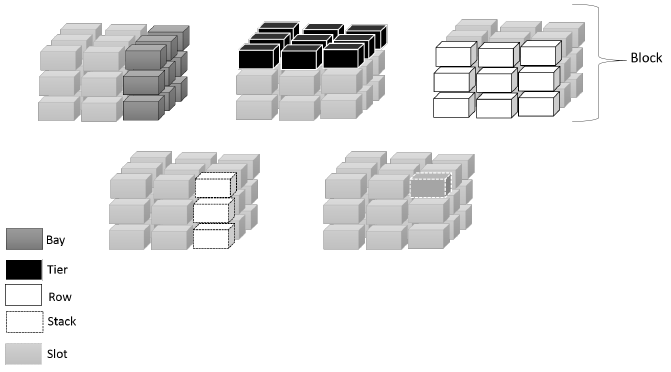
Figure 1 depicts a containers yard where each block is composed by a group of rows, tiers, and bays. The intersection of a specific row and bay of a block indicates a stack in a two-dimensional schema, in contrast to the traditional schema with three dimensions row, tier, and bay. The three-dimensional schema allows us to represent the specific position or slot of a container within a block of the yard from the intersection of a row, tier, and bay coordinates. Nevertheless, a two-dimensional schema decreases the problem complexity for an optimized computational solution.
The objective of a container storage space allocation strategy depends on the type of container and the information available on it. Therefore, the studies that analyze this optimization problem usually specify these aspects. The import containers are usually downloaded from ships or trains in large groups and retrieved by individual customers in small numbers. The departure date from the yard is usually unknown.
The export containers flow is different to the import containers flow because the arrival date is often unknown, but its departure date is relatively fixed. The loading sequence of the export containers depends on the weight of each container, among other information [3].
Strategies for storage space allocation develop solutions for individual containers or groups of containers. The storage space allocation for individual containers is about assigning the containers to yard blocks and assigning them specific positions within the selected block. The second strategy deals with assigning groups of containers to storage locations, where the groups could be on their target vessel, owner, destiny, among other features. Authors Bazzazi et al. [1] explained that the SSAP can be formulated as a generalized assignment problem. They also explained that the SSAP belongs to the category of NP-Hard problems.
In this paper, we model SSAP as a generalized assignment problem for import container, and we assign individual positions to each container within a specific block. We have an input container arrival sequence (c 1 , c 2 … c n ), where each container c n has a known arrival and departure date. We know the cost of assign every container to each position. The outputs of the optimization method are the positions for each container (s, t, c), where s is the stack, t is the tier in this stack, and c is the container in this stack and tier.
3 Related Work
The authors Kim and Kim published one of the pioneer papers dealing with import containers in 1999 [9]. In this paper, the authors proposed a segregation strategy to store containers. Their strategy allocates storage spaces for each newly arriving container in a vessel and prohibits to mix container discharged from different vessels. Their goal was to minimize the number of expected reshuffles when delivering the containers, but they did not optimize efficient exploitation of the storage yard.
The authors Kim and Kim [10] presented a mathematical model to obtain the optimal container stacking plan in a terminal where there is a limited free storage time for import containers. The containers which stay too long time in the yard have to pay storage costs. The goal of this work is "to minimize the number of reshuffles by minimizing the dwell times of containers."
In [19] the authors Saurí and Martin proposed three strategies to determine minimum reshuffles in an import container terminal by a probabilistic based mathematical model. The authors found out that the optimal strategy depends on the stacking height and the relationship between vessel headway and container dwell time.
Several cases have been proposed using GA, among them in [15,11,1,20,14,21]. The authors Park and Seo in the article [15] solved the planar storage location assignment problem, which consists in to store import and export containers by minimizing the number of obstructive object movements or reshuffles. The authors proposed a mathematical model and a GA to solve the problem.
The authors Kozan and Preston in [11] proposed an iterative search algorithm that includes a transfer model and an assignment model. The algorithm cyclically determines the optimal storage locations for import and export containers. They also proposed a GA, a tabu search algorithm, and a hybridization of these two algorithms.
The authors Bazzazi and Javadian in [1] proposed a GA to solve the SSAP by considering container types like regular, empty, refrigerated, dangerous, etc. Their optimization objective was to balance the workloads between blocks to minimize the time required to store or to retrieve containers.
Authors Park et al. [16] proposed a two-step algorithm. The algorithm dynamically allocates stacking positions to containers in an automated container terminal. They decided the best block for an incoming container in the first step, and in the second step, they selected the proper stacking position of an import container within a block.
Sriphrabu et al. [20] solved a simulation model for stacking containers applying a GA. They minimize the total lifting time and increased service efficiency of the container terminals. They showed the suitable containers location assignment based on the arrival of containers at a container terminal.
Furthermore, they correlated it with the order of the containers loaded onto container ships.
Ndiaye et al. [14] proposed a linear mathematical model which assigned an accurate storage location to every import containers. They considered a container terminal which uses straddle carriers (SCs) as transfer and handling equipment and aimed to minimize simultaneously the number of reshuffles and the total distance traveled by the SCs between the quays and the storage yard. The authors proposed an ant colony algorithm, a bee algorithm, and two hybridizations for numerical resolution.
Authors Yang et al. in [21] presented the container Stacking Position Determination Problem (SPDP) under the mode of loading and unloading operations. They solved the SPDP by a multi-objective programming model. The objective combines the maximization of the container circulation moreover, the minimization of unbalance workloads. Then, they developed a GA to solve the problem.
Boysen and Emde in [2] formalized the parallel stack loading problem (PSLP). In this kind of decision problem, a given stream of items is successively stored in multiple parallel stacks with limited capacity, such that blockages. The blockages are, for example, items with lower priority stacked on top of items with departure date early. In this work, the blockages are minimized. The authors showed the PSLP computational complexity and presented an exact and heuristic solution.
Although there are several solutions for SSAP, none of the mathematical models fit the real containers yard analyzed in this paper. The schema of the real yard under modeling is in Figure 2. The existing solutions are for containers yards with larger dimensions, different types of equipment, flow, and objective to be optimized. In the containers real Cuban yard, the operators employ a reachstacker crane for stacking operations.

Fig. 2 Diagram of the real containers yard analyzed in our work. Currently, the containers yard has six rows with three access vials, and three tiers by stack. The number of stacks by rows varies depending on the sizes of the containers
For this type of equipment, in the physical conditions of the containers yard is difficult to access the first row of containers in the yard due to the existence of a fence. To access to this row of containers, the operator must perform unproductive movements in the second row. However, the slots in the first row should continue in use, to avoid the wasting of storage space. These characteristics of the containers yard demand a new solution, which takes into account these requirements.
4 Mathematical Programming Formulation
In this section, we present a 0-1 integer linear programming formulation to solve SSAP to import container flow. We highlight our assumptions before the description of the mathematical model.
4.1 Assumptions
We suppose that:
- We know the date of departure, the size, the customer, and the destination of each container.
- The size of the containers can be 20 or 40 feet.
- We take into account the containers already stored in the yard.
- We assign containers to slots according to the dimensions of each one.
- We consider a multi-modal container terminal, which means that an import container can arrive at the yard by train or truck and to leave by truck.
- The yard is organized in rows, where each row contains several stacks and these are formed by tiers.
- The intersection of a specific stack and tier is considered a slot.
- We consider a small container terminal; containers are stacked and transported by one reachstacker.
- The reachstacker cannot access directly to the first row of the yard because it is next to a fence. The reachstacker to stack a container in the first row, usually perform unproductive moves in the second row.
4.2 Indices and Parameters
Indices
s: stack.
t: tier.
c: container.
Parameters
N s : The total number of stacks in the yard.
T: The total number of tiers in every stack.
N c : The total number of import containers to stack.
S s : Size of stacks s.
T c : Departure date of arrival container c.
S c : Size of the container c.
Ccs,t: Cost of assign the position s, t to container c.
M: A big integer.
Decision Variable
4.3 Mathematical Model
The objective function is to minimize the value of Z represented by the mathematical expression in (1). The objective function minimizes the number of expected reshuffles of the reachstacker when unloading the containers. We use a cost matrix Ccs,t as a parameter of the objective function. The cost matrix contains the cost of stacking each new container of the input sequence (c 1, c 2, …, c n ) to each position on the yard (s, t). Positions previously assigned to another container are not available and receive a very high cost (M) in the matrix.
The positions at first row of the yard are difficult to access the reachstacker. Therefore, corresponding values to the first row in the cost matrix have an initial cost of five. For the remaining positions in the yard, the cost is ten for each reshuffle generated, or zero if there is not any reshuffle. Hence, the cost of a reshuffle in row one is higher than another position of the yard. However, a container assigned to a position in the first row but without generating reshuffles has a cost of five, lower than another position which generates a reshuffle. In this case, it will always be preferable to stack it on row one. This decision responds to the need to efficiently use the yard's space, even though what it is desirable to minimize the number of unproductive movements of the reachstacker:
The model is subject to:
Constraints in the mathematical expression (2) state that each position can storage at most one container. Constraints in expression (3) state that each container must be assigned exactly to one position. Constraints in expression (4) state that the containers should be not in the air, which means that a container should be allocated over another container and not over an empty slot. Constraints in expression (5) state that no container must be assigned to an occupied position in the yard. Constraints in expression (6) state that all containers have to be assigned to a stack of the same size. Finally, the last constraints in expression (7) state that the arrival containers should be ordered descending by their departure dates.
The first three sets of constraints (2), (3), and (4) are also posed by the authors Park and Seo [15,14]. In addition Ndiaye et al. [14] defined constraints similar to our constraints in expression (5). They also assumed that the yard has occupied positions before the new containers arrive, in their mathematical modeling. Authors Ndiaye et al. [14], and Bazzaziet al. [1] also defined constraints similar to our constraints in expression (6). Usually, these constraints depend on the policies established by the containers yard operators. Finally, the sixth constraints have been used by Ndiaye et al. in [14]. However, the objective function present by Ndiaye et al. [14] differs from the objective function of the present study, among other aspects of its mathematical modeling.
5 Exact Solution and Computational Experiments
We write the SSAP in GNU Math-Prog language. The hardware setup includes an Intel Core i7-3520M, processor at 2.90 GHz and 8GB of RAM.
We collect the data from the yard operations for the last four years and organize them into four datasets, to validate the efficiency of the optimization method. Every instance in the dataset represents a container to stack in the yard with their respective date of arrival, size, customer, destination, and departure date.
Since the optimization method used gives an exact solution in all cases where it exists, it is needless to evaluate the accuracy of the solution. In contrast, we measure the efficiency of the optimization method regarding its computational time.
When the containers arrive at the yard, they are downloaded to the platform. This operation takes one hour for 25 containers. For this reason, we assume that the solver should solve the model in less than 3600 seconds. Initially, the containers yard is:
- Empty.
- Partially filled with some empty slots higher than the number of containers to stack.
- Partially filled with some empty slots less than the number of containers to stack.
- Full.
The two initial configurations generate valid solutions. However, for the last two configurations, there is no solution in this work. The decision to make when any of the last two situations occur will be addressed in further work.
We divide the data into four datasets to create four cases of study:
- Dataset 1. It contains instances describing the current conditions of the storage yard, 45 stacks and 3 tier height in each one. It only varies from one instance to another the number of containers to stack, the number of stacks in the first row and the initial yard configuration. The initial yard configuration represents the occupied and empty positions in the yard.
- Dataset 2. It contains instances that describe a further situation in which the storage area of the containers expands, increasing the number of stacks to 90 stacks and the same number of tiers of the dataset 1.
- Dataset 3. It contains instances of the further variant in which the tiers of the stacks are increased up to 4 and 5 levels, and the number of stacks is 45 same dataset 1.
- Dataset 4. It contains instances of the further variant in which the yard policies on the tiers increased up to 4 and 5 levels, and the number of stacks increases to 90 same dataset 2.
We represent the instances in each of the datasets as a 5-element tuple. These elements are:
Initial yard configuration,
Number of stacks in the first row,
Size of each stack,
Containers already stacked in the yard,
Containers to stack.
Table 1 shows two examples of instances of the structure of the dataset. The initial-yard-configuration is a list of stacks. The value 1 indicates an occupied slot while 0 an empty slot. By knowing the number of stacks in the first row, we penalize the assignment of containers to this row where is difficult the access of the reachstacker.
Table 1 Example instances of the structure of the dataset for import containers SSAP
| Container 1 | Container 2 | |
|---|---|---|
| Initial Config | [110][100][111][000] | [111][000][111][000] |
| Stack # First row | 2 | 2 |
| Stack size | [20,20,40,20] | [20,40,40,20] |
| Stacked containers | [[15/2/17, 18/2/17,0] | [[15/2/17,18/2/17,1/1/17][0,0,0] |
| [1/1/17,0,][1/1/17,15/1/17, | [1/1/17,15/1/17,18/1/17][0,0,0]] | |
| 18/1/17][0,0,0]] | ||
| Containers to stack | [[Size,Departure,Clie,Dest], | [[Size,Departure,Clie,Dest], |
| [Size,Departure,Clie,Dest] | [Size,Departure,Clie,Dest] | |
| […]] | […]] |
The stack-size is a list of two possible values 20 or 40, allowing 20-feet or 40-feet containers. The stacked-container is a list similar to the initial configuration, but for the occupied positions has the departure date of the container. The containers-to-be-stacked is a container list with a 4-elements tuple [Size, Departure Date, Client, Destiny]. The last two elements of the containers-to-be-stacked are needless in this work. However, they are needed for further work.
Table 2 presents a description of the instances by datasets. Each cell contains the number of containers stacked in the yard, the number of stacks in the first row, and the number of containers to stack. An asterisk next to the number of stacks in the first row indicates occupied slots. If the number of stacked containers is 0, then the containers yard is initially empty (e.g., first instances of all datasets). Also, there are instances with an equal number of stacked containers, containers to stack, and stacks in the first row. However, these instances differ in the initial configuration of the yard (e.g., instances four and five of the dataset one).
Table 2 Description of the instances by datasets [Stacked containers#, Stack#First row, Containers to stack #]
| Instance | Dataset 1 | Dataset 2 | Dataset 3 | Dataset 4 |
|---|---|---|---|---|
| 1 | [0,5,135] | [0,15,270] | [0,10,180] | 0,15,360 |
| 2 | [60,5*,45] | [0,15,200] | [0,10,225] | 50,15*,180 |
| 3 | [54,5,50] | [50,15,200] | [0,10,100] | 0,15,450 |
| 4 | [25,5,100] | [50, 15*,200] | [0,10,200] | 50,15*,300 |
| 5 | [25,5*,100] | [100,15*,170] | [100,10,60] | 72,15,150 |
| 6 | [0,5,50] | [100,15*,150] | [100,10*,60] | 100,15*,150 |
| 7 | [0,5,100] | [100,15*,150] | [140,10,50] | 50,15,300 |
| 8 | [30,10*,100] | [100,15*,150] | [140,10*,50] | 50,15,200 |
| 9 | [30,12*,100] | [170,15*,60] | [140,10*,25] | 100, 15*,240 |
| 10 | [51,10*,75] | [170,15*,60] | [100,10, 35] | 100,15*,300 |
5.1 Solver Selection
We experiment with two free and open source solvers for linear mixed-integer programming:
The programming language used to develop GLPK and LPSolve is ANSI C. Also, both accept files in MPS, GNU MathProg, and CPLEX LP format. GLPK uses the Dual and Primal Revised Simplex and Interior Point methods for linear problems. Additionally, uses Branch and Cut method for mixed-integer linear programming problems, which is a hybrid of Branch and Bound and cutting plane methods. lpSolve uses Dual and Primal Revised Simplex method for linear optimization problems like GLPK, but for mixed-integer programming uses the Branch and Bound method.
In our experiments, lpSolve takes a long time to solve 22 instances of all dataset (See Figure 4). Therefore, we consider that lpSolve solver computational time unacceptable for current yard conditions or further situations.

Fig. 4 Graph of the computational times employed by the lpSolve solver to optimize all instances of all datasets
Figure 5 shows the computational times for the instances of the four datasets with the GLPK solver. For the instances that represent the current conditions of the yard (dataset 1) the computational times do not exceed one second, which is considered acceptable (See Figure 5a).

Fig. 5 Graph of the Computational Times Employed by the GLPK Solver to Optimize the SSAP problem. a) Graph for instances of the dataset 1 corresponding to the current conditions of the containers yard. b) Graph for instances of the dataset 2 corresponding to further conditions of the containers yard. b) Graph for instances of the dataset 3 corresponding to further conditions of the containers yard. b) Graph for instances of the dataset 4 corresponding to further conditions of the containers yard
For the further conditions of the yard, represented in dataset 2, the longest time is approximately four seconds corresponding to the first instance (See Figure 5b). Computational times for instances of the dataset 3 do not exceed three seconds, in contrast to the four and six instances that exceed the acceptable computational time. However, the computational times for the instances of dataset 4 are higher (See Figure 5d). In this dataset, GLPK needs more than 3600 seconds to solve the model represented in four instances. We consider acceptable the computational time of the optimization method with the GLPK solver for the two first dataset. Nevertheless, the third and fourth dataset computational time is unacceptable.
Figure 3 summarizes the results of the computational times of the GLPK solver for the 40 instances. The computational time grows according to the yard dimensions. As a consequence, we conclude that the proposed optimization method solved with the GLPK is acceptable for the current conditions of the yard moreover, for further conditions described in dataset 2. Hence, we select the GLPK to solve the SSAP for the real Cuban yard. Our selection responds to four reasons. First, the GLPK solves the SSAP in an acceptable computational time according to our experiments. Second, GLPK is one of the most popular free and open source solver [12]. Third, it is available for the different operating system. Fourth, GLPK solves optimization problems without dimensional restriction. However, the proposed solution is impractical for the configuration described in the dataset 3 and 4. Therefore, it is necessary to analyze other optimization methods that perform the stacking with a cost close to the optimum but in a shorter computational time. In the next section, we analyze a solution with GA metaheuristic.

6 Genetic Algorithm Implementation
Genetic algorithms are search methods inspired by the natural selection [7]. In the GA, unlike the exact methods, the decision variables of the problem are encoded as an individual, which represents a candidate solution, also known as a chromosome in genetic terms. A fitness function compares chromosomes regarding their profits, similar to the objective function for exact methods. In GA, the term population is a set of candidate solutions or chromosomes. Unlike the exact methods, which find the optimal solution to an optimization problem even with high computational time, GA find solutions close to the optimum (suboptimal solutions) however, with lower computational time. Therefore, we implement a GA in order to find suboptimal solutions to the SSAP for the instances of datasets 3 and 4 with acceptable computational time.
GA follows the following steps to search suboptimal solutions [6]:
Next, we describe our representation of the SSAP and the solution with a GA. We present the genetic operators and the parameters with the best performance for each dataset. Additionally, we show the computational time for each dataset.
6.1 Chromosome Representation
To represent the chromosome for the SSAP, we use the number of containers to be stacked and the number of available positions in the containers yard.
Figure 6 shows the representation of the chromosome obtained as the suboptimal solution, for instance nine of dataset three. The position index in the chromosome corresponds to the index obtained by sorting the available positions in the containers yard, which is not the position in the containers yard. The length of the chromosome is determined by the number of containers to be stacked.

Fig. 6 Chromosome representation for containers SSAP. First row indicates the length of the chromosome, that is the number of containers to be stacked. Second row represents the assigned available position index. For example, in first column 1 is the first stacked container and 75 is the assigned position by the GA metaheuristic
For example, a chromosome with length 25 corresponds to 25 containers to be stacked. The possible values assigned to each gene of the chromosome are the available positions in the containers yard sorted as we previously described. For example, for the chromosome in Figure 6, each gene could take a value between one and 85, because there are 85 available positions.
With this representation of the chromosome, we do not need the constraints (2), (5), and (7) of the mathematical model. The number of containers determines the length of the chromosome. Therefore, there is always one container by position, and there are not two containers assigned to the same position. However, it is possible to obtain a chromosome with a container assigned to two positions. Hence, we include the constraint (3).
This representation also guarantees that the containers are not assigned to positions that are not available (Constraint (5)).
6.2 Parent Selection
As selection operator, we use the Roulette Wheel Selection [13] is chosen 40% of the time, and Tournament Selection [13] with a size of two and chosen 60% of the time. Our fitness function computes the cost of stacking each container on each of available position. This cost is measured regarding reshuffles. The fitness function also includes three constraints 3, 4, and 6 as penalizations. So that, a chromosome is valid as long as it does not violate any of these constraints. Moreover, a chromosome is best-performed as long as it does not violate the constraints and the cost is small.
6.3 Crossover
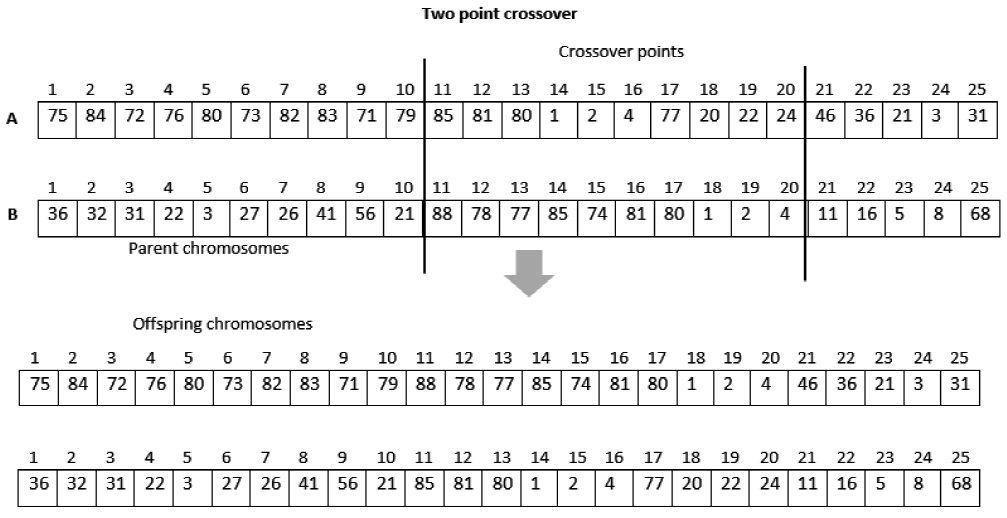
In the actual scientific literature many crossover operators have been designed, for example, by the authors Raj Singh et al. in [18]. However, according to our chromosome representation, we decided to employ the two-point crossover random crossing operator by Goldberg et. al [6]. Thus, we avoid a greater repetition of genes in the child chromosomes, which it conduces to a constraint violation. Figure 7 shows an example of two parent chromosomes crossed using the two-point crossover and forming two new chromosomes. We use a different crossing probability for each dataset: for dataset 2 and 3 - 0.2, for dataset 1 -0.4, and for dataset 4 - 0.45.
As we mentioned before, the datasets respond to the current physical conditions of the containers yard (dataset 1) and variants of possible growth of the containers yard in horizontal and/or vertical directions (dataset 2, 3, and 4). Therefore, we adjust the GA parameters for each particular dataset.
6.4 Mutation
We implement the mutation through an operator that exchanges two genes of a chromosome (Swap Mutation) [4]. The chromosomes of the population are mutate with a certain probability: 0.05 for all dataset in our research. First, we determine which chromosomes will mutate using the previous probability. Second, for the chromosomes that will mutate, we generate two random numbers in the range between one and the size of the chromosome. These numbers correspond to two containers to which we exchange their positions. For example, Figure 8 shows the mutation between genes seven and 17 in a chromosome, this means that the positions of both containers must be exchanged.

In the new chromosome, container seven occupies position 51 and container 17 occupies position 82. This mutation operator allows us to generate a new chromosome that meets most of the constraints as the original chromosome. Other mutation operators, more common, do not achieve this advantage.
6.5 Numerical Experiments
Our solution, using GA, is implemented in ECJ3 for all datasets, which is an evolutionary computation framework written in Java. Similarly, all the computational experiments are executed on the same hardware used for the experimentation with the exact methods. We generate the initial population of candidate solutions randomly across the search space. The population size for each dataset was different, to explore a big number of solutions according to the size of the yard. For dataset 1 we define 2000 chromosomes, while in the other datasets, we define 2000, 3000, and 8000 chromosomes. Like the population size, the number of generations allows generating better chromosomes, although it can mean an increase of the computational time [6]. We use between 2000 and 3000 generations for different datasets, which a big generations number. However, Figure 9 shows that the computational times were acceptable for all the instances analyzed. For cases where more containers are stacked (instances 8, 9, and 10 of the last dataset) the computational times did not exceed 1020 seconds achieving suboptimal solutions. In the next section, we discuss the results obtained from the implementation of the GA and the exact method that gave the best results for the SSAP for the containers yard.

7 Results Discussion
For containers yard operators, it is important to obtain the container stacking plans in acceptable computational time for the correct execution of the operations in the containers yard. Also, operators need solutions that minimize the number of reshuffles, for the saving of their resources.
Hence, in this paper, we explore three solutions for SSAP:
- Solver lpSolve with Branch and Bound method.
- Solver GLPK with Branch and Cut method.
- GA metaheuristic with ECJ framework.
On the one hand, solutions with the Branch and Bound method and the solver lpSolve did not satisfy the computational time for any of the datasets. Our claim is based on the fact that a lot of instances of the four datasets exceeded the acceptable computational time. Nevertheless, the exact method with the GLPK solver obtained better results; but, it did not find an optimal solution in the computational time acceptable for some of the instances that represent further growths of the containers yard.
GA metaheuristic with the ECJ framework allowed us to explore the search space differently. Therefore, GA found suboptimal solutions for all instances in acceptable computational time. Although GA obtained solutions with reshuffles than exact methods for most of the instances, it managed to find solutions to all the instances in the computational time defined as acceptable, 3600 seconds.
Figure 10 shows the computational times for all instances solved with GA and the exact method with GLPK solver. GA's computational times are lower for most of the instances. When the exact method with the GLPK solver took longer than the acceptable time, the GA did find a suboptimal solution. Is worth to say that, although the GA achieved better results than the exact method regarding computational time, its solutions cause a more number of reshuffles (See Table 3).

Fig. 10 Graph of the computational times employed by ECJ (GA) and GLPK (Branch and Cut) to compute all instaces corresponding to each configurations of the containers yard
Table 3 Expected containers reshuffles number all instances with GA metaheuristic and GLPK solver. It has been marked with 0* those instances where the GLPK did not find the solution in the acceptable computational time and with an unknown number of reshuffles
| Dataset | Method | Intance | |||||||||
|---|---|---|---|---|---|---|---|---|---|---|---|
| 1 | 2 | 3 | 4 | 5 | 6 | 7 | 8 | 9 | 10 | ||
| 1 | GLPK | 0 | 14 | 9 | 4 | 4 | 0 | 0 | 12 | 12 | 32 |
| GA | 0 | 20 | 13 | 11 | 15 | 0 | 0 | 17 | 18 | 27 | |
| 2 | GLPK | 0 | 0 | 39 | 39 | 80 | 58 | 56 | 56 | 44 | 42 |
| GA | 0 | 0 | 83 | 73 | 100 | 88 | 91 | 91 | 51 | 50 | |
| 3 | GLPK | 0 | 0 | 0 | 0* | 44 | 0* | 27 | 30 | 30 | 44 |
| GA | 0 | 0 | 0 | 0 | 76 | 76 | 47 | 57 | 40 | 51 | |
| 4 | GLPK | 0 | 0* | 0 | 0 | 0 | 0 | 0 | 0* | 0* | 0* |
| GA | 0 | 25 | 0 | 259 | 97 | 121 | 206 | 80 | 249 | 250 | |
Also, when the containers yard is initially empty, both the GLPK and the GA, find the best solution with zero reshuffles. From these results, we conclude that the operators of the containers yard must use the exact solution for the current situation and the growth of the containers yard represented in dataset 2. While for the other conditions studied, corresponding to other growths of the containers yard, they must use the metaheuristics GA.
8 Conclusion
This paper presented the mathematical model for the SSAP for an import containers yard. We modeled the optimization problem as a generalized assignment problem. Next, we solved the mathematical model using exact optimization methods validating it by several experiments performed on data from an import containers yard. The instances used in the experiment were grouped into four datasets according to different configurations of the containers yard.
From our experiments, we found that the Branch and Cut method with solver GLPK achieved better results than the lpSolve, regarding the computational time. Moreover, we noticed that the SSAP for the current containers yard could be solved with a mixed-integer linear programming method in the acceptable computational time defined. However, this method was not feasible for the projected growths of the containers yard.
For the growths of the containers yard, we explore the metaheuristics GA using the ECJ framework. We adjust the GA's main parameters for each dataset, such as population size, generations, mutation, and crossover probabilities. Finally, we found that for the current dimensions of the containers yard, represented in dataset 1 and 2, GLPK solved them in acceptable computational time, always finding the optimal solution. However, for instances 4 and 6 of dataset 3 and instances of dataset 4, it was the GA who resolved all instances in acceptable computational time. Therefore we suggest a mixed solution of both methods, depending on the size of the containers terminal.
As further work, we propose to analyze the behavior of these optimization methods adding some other constraints. For example, stacking containers with different sizes in the first and second yard row, grouping containers attending to their customers and destination, and partial fulfillment of the containers yard with some of empty slots less than the number of containers to be stacked.

