


 text new page (beta)
 English (pdf)
 Article in xml format
 Article references
 Send this article by e-mail
 Cited by SciELO
  Similars in
SciELO
Similars in
SciELO 
 Permalink
1 Introduction
In the last decades, robotic rovers, such as the Mars Exploration rover Opportunity [1, 2] and the Mars Science Laboratory’s rover Curiosity [3, 4], have proven to be very powerful and long lasting tools for Mars exploration due to their ability to navigate and perform activities semi-autonomously [5], as well to survive beyond any prediction [6], which have allowed them to get a closer look at any interesting target found in their path and to further extend the territory explored [7, 8]. The activities to be performed by the rover during the day are usually instructed only once per Martian day (often called a sol) via a prescheduled sequence of commands, which are sent each morning by the scientists and engineers on Earth [9]. A sol is just about 40 minutes longer than a day on Earth. The rover is expected to safely and precisely navigate along a given path, position itself with respect to a target, deploy its instruments to collect valuable scientific data, and return them back to earth [5], where any kind of navigation error could result in the loss of a whole day of scientific exploration, trap the vehicle in hazardous terrain, or damage the hardware [7, 8]. On Earth, the data received will be used for scientific research and to plan the next sol’s activities [9].
For safe and precise autonomous navigation, the rover must know its exact position and orientation during the execution of all motion commands [10]. The rover’s position is estimated by integrating the rover’s translation over time, which in turn is estimated from a combination of encoder readings of how much the wheels turn (wheel odometry) with heading updates from the gyros [11]. The position at the beginning of the rover’s motion is assumed to be known or reset by command. The rover’s orientation is estimated by integrating the rover’s rotation over time, where the latter is delivered by gyros of an Inertial Measurement Unit (IMU) onboard the rover [11]. The initial orientation of the rover is estimated from both accelerometer measurements delivered by the IMU and the position of the sun, which is obtained by a sun sensor that is also part of the rover navigation system [12].
A common problem associated with the use of wheel odometry is that the accumulated error of wheel odometry with distance traveled highly depends on the type and geometry of the terrain over which the rover has been traversing, being small on level high friction terrain [13, 11, 8], where the wheel slip is small due to good traction, and large on steep slopes and sandy terrain [10, 7, 14], where the wheels slip due to the loss of traction or when a wheel pushes up agains a rock [13]. This limits the autonomous navigation of the planetary rovers on slippery environments [15], because the position estimate derived solely from wheel encoders would not be very accurate to be trusted to compensating for slip in order to ensure that the rover stays on the desired path [10]. In addition, the excessive wheel slip could even cause the rovers to get stuck in soft terrain [10, 16].
In order to improve the safety and autonomous navigation accuracy of rovers in slippery environments, the rover is often commanded to perform the correction of any error that occurred because of wheel slippage after moving a small amount by using the rover’s position estimate, which is determined by a feature based stereo visual odometry algorithm [10, 17, 5]. This algorithm is able to determine the rover’s position and orientation from the video signal delivered by a stereo video camera mounted on the rover [18]. It can be roughly summarized in seventh steps. In the first step, a stereo pair is captured before the rover moves and a set of 2D feature points are chosen carefully evenly across the left image. In the second step, the 3D positions of the selected 2D feature points are estimated by establishing 2D feature point correspondences and using triangulation to derive the 3D positions [19]. In the third step, after the rover moves a short distance, a second stereo pair is captured.
Then the previously selected 2D feature points are projected onto the second stereo pair by using an initial motion estimate provided by the onboard wheel odometry. In the fourth step, the projected 2D feature point positions are refined and their 3D positions are also estimated by establishing 2D feature point correspondences and using triangulation to derive the 3D positions. In the fifth step, the 3D correspondences between the set of 3D feature point positions computed before the rover’s motion and the set of 3D feature point positions computed after the rover’s motion are established. In the sixth step, the conditional probability of the established 3D correspondences is computed and then maximized to find the 3D motion estimates. Finally, in the seventh step, the motion estimates are accumulated over time in order to get the rover’s position and orientation.
The above algorithm was initially described in [20], then it was further developed in [21, 22, 23], until a real-time version of it was implemented and incorporated in the rovers Spirit and Opportunity of the Mars Exploration Rover Mission [10]. After evaluating its performance in both Spirit and Opportunity rovers on Mars, changes were made in [24] to improve its robustness and reduce the onboard processing time. This last updated version of the stereo visual odometry algorithm is currently being used in the Curiosity rover [25, 26].
There are other similar algorithms in the professional literature [27, 28, 29, 30, 31, 32], which have even been adapted for to operate with a monocular [30] or an omnidirectional video camera [33, 34, 35, 36], and recently, extended to Simultaneous Localization and Mapping (SLAM) [37, 38]. Refer to [39, 40] for a comprehensive tutorial on visual odometry.
In [41, 42], a monocular visual odometry algorithm based on intensity differences was proposed as an alternative to the long-established feature based stereo visual odometry algorithms, which avoids having to establish 2D and 3D feature points correspondences for motion estimation, tasks that are known to be very difficult, to consume a lot of processing time [27] and are prone to match errors due to large motions, occlusions or ambiguities, which greatly affect the 3D motion estimation [21]. With this algorithm it is possible to estimate the 3D motion of the rover by means of the maximization of the conditional probability of the intensity differences measured at key observation points between two successive images. The images are taken by a single video camera prior to and after the motion of the rover. The key observation points are image points whose linear intensity gradients are found to be high.
Although the starting point to compute the conditional probability is the well known optical flow constraint [43, 44], this is not a typical two-stage 3D motion estimation algorithm as those described in [45, 46, 47, 48, 49, 50, 51, 52, 53], which requires the estimation of the optical flow vector field as an intermediate step, but rather a one-stage 3D motion estimation algorithm similar as those proposed in [54, 55, 56, 57, 58, 59, 60], which is able to directly deliver the 3D motion just evaluating intensity differences at key observation points, thereby avoiding in this way solving the ill-posed problem of optic flow estimation, whose solution is rarely unique and stable [61].
Despite that in [41, 42] the above intensity-difference based monocular visual odometry algorithm has been extensively tested with synthetic data to investigate its error growth at different intensity error variances, an experimental validation of the algorithm in a real rover platform in outdoor sunlit conditions is still missing. Therefore, this paper’s main contribution will be to provide that missing validation data to help to clarify whether the algorithm really does what is intended to do in real outdoors situations. However because the terrain shape is unknown, flat terrain will be assumed and the results presented in this contribution will be from experiments conducted only on flat ground.
Since the final goal of the algorithm is for it to be used in the rover’s positioning, its positioning performance will be assessed for validation, where the absolute position error of distance traveled will be used as a performance measure. Minimal, it is expected to obtain an absolute position error within a range of 0.15% and 2.5% of distance traveled, similar to those achieved by traditional feature based stereo visual odometry algorithms [45, 28, 10, 30, 34], which have been successfully used in rovers here on Earth and on Mars. The processing time per image will be also reported.
This contribution is organized as follows: in section 2, the monocular visual odometry algorithm is briefly described; in section 3, the experimental validation results are presented; and finally, in section 4, a summary and the conclusions are given.
2 Visual Odometry Algorithm
This algorithm is able to estimate the rover’s 3D motion from two successive intensity images I k−1 and I k . The images depict a part of the planet’s surface next to the rover and are taken by a single video camera at time t k−1 and time t k , which has been mounted on the rover looking to one side tilted downwards to the planet’s surface. The estimation is achieved by maximizing a likelihood function consisting of the natural logarithm of the conditional probability of intensity differences at key observation points between both intensity images. The conditional probability is computed by taking as a starting point assumptions of how the world is constructed and how an image is formed.
Subsections 2.1 and 2.2 describe these assumptions. The conditional probability is computed in subsection 2.3. In subsection 2.4, the method for maximizing the natural logarithm of the conditional probability to determine the rover’s 3D motion is explained.
2.1 Motion, Camera and Illumination Models
The rover’s 3D motion from time t k−1 to time t k is described by a rotation followed by a translation of its own coordinate system (q, r, s) with respect to the fixed surface coordinate system (X, Y, Z). The translation is described by the 3 components of the 3D translation vector ∆T = (∆T X , ∆T Y , ∆T Z )⊤.
The rotation is described by 3 rotation angles: ∆ω X , ∆ω Y , ∆ω Z . Here, the unknown six motion parameters are represented by the vector B = (∆T X , ∆T Y , ∆T Z , ∆ω X , ∆ω Y , ∆ω Z )⊤. In addition, the rover coordinate system (q, r, s) and the camera coordinate system are supposed to be the same, and the camera coordinate system (q, r, s) is supposed to coincide with the fixed surface coordinate system (X, Y, Z) at time t 0.
Thus, the accumulated 3D motion of the surface with respect to the camera coordinate system (q, r, s) is the accumulated negative 3D motion of the rover with respect to the fixed coordinate system (X, Y, Z). Furthermore, it is assumed that an image is formed through perspective projection onto the camera plane of that part of the surface next to the rover, which is inside the camera’s field of view. That part is called herein the visible part of the surface. Moreover, it is assumed that there are no moving objects on the visible part of the surface and that the surface is Lambertian, as well as the illumination is diffuse and time invariant. Thus, the intensity difference at any key observation point is due only to the rover’s 3D motion.
2.2 Surface Model
For 3D motion estimation from time t k−1 to time t k , the 3D shape of a rectangular portion of the visible part of the surface and its relative pose to the camera coordinate system (q, r, s), as well as a set of observation points are supposed to be known at time t k−1 . The 3D shape of this rectangular surface portion is assumed to be flat and rigid and described by meshing together two triangles, forming the rectangle. The pose is described by a set of six parameters: the three components of a 3D position vector and three rotation angles. An observation point lies on the rectangular surface portion at barycentric coordinates A v and carries the intensity value I, as well as the linear intensity gradients g = (g x , g y )⊤ at position A v . From now on, these known shape, pose and observation points will be referred as the surface model at time t k−1 . The surface model at time t k−1 is obtained by moving (rotating and translating) the surface model from its pose at time t k−2 to the corresponding pose at time t k−1 with the negative of the rover’s 3D motion estimates from time t k−2 to time t k−1 . The initial surface model at time t 0 is currently created and initialized a priori during the time interval extending from time t −a until time t 0: [t −a , t −a+1 ,..., t −b ,..., t −c ,..., t −d ,..., t −1, t 0].
During this initialization time interval the rover does not move. Thus the surface model’s pose remains constant in that interval.
2.2.1 Shape Initialization
The dimensions of the rectangular flat surface model are initialized with the same dimensions as a real planar checkerboard pattern, which is placed on the surface in front of the camera at time t −b and removed from the scene at time t −d during the initialization time interval. The pattern is placed so that its perspective projection onto the camera plane lies in the center of the image and covers approximately 20% of the total image area. The pattern has 8x6 squares of 50 mm side length.
2.2.2 Pose Initialization
The pose of the initial surface model with respect to the camera coordinate system (q, r, s) is set equal to the position and orientation of the real pattern mentioned above with respect to the camera coordinate system. The position and orientation are estimated in two steps during the initialization time interval. First, an intensity image I −c of the real pattern on the surface is captured at time instant t −c , where t −b < t −c < t −d . Then, the position and orientation are estimated by applying Tsai’s coplanar camera calibration algorithm [62] to the intensity image I −c . The pattern is removed from the scene after calibration at time instant t −d . The camera calibration also ensures metric motion estimates.
2.2.3 Observation Points Initialization
The observation points of the initial surface model are created and initialized in five steps at the end of the initialization time interval by using the intensity image I 0 captured at time t 0. First, the gradient images G 0x and G 0y are computed by convolving the intensity image I 0 with the Sobel operator. In the second step, the image region of each triangle of the surface model is computed by perspective projecting their 3D vertex positions into the camera plane. In the third step, the observation points are selected but only inside the image regions of the projected triangles. An arbitrary image point a inside the image region of a projected triangle will be selected as an observation point only if the linear intensity gradient at position a satisfies |G0(a)| > δ 1.
This selection rule will reduce the influence of the camera noise and increase the accuracy of the estimation. The value of the threshold δ 1 was heuristically set to 12 and remains constant throughout the experiments. In the fourth step, the 3D positions of the selected observation points on the model surface with respect to the camera coordinate system are computed. The 3D position vector A of an arbitrary selected observation is computed as the intersection of the a’s line of sight and the plane containing the corresponding triangle’s vertex 3D positions. The corresponding barycentric coordinates A v with respect to the vertex 3D positions are also computed. Finally, in the fifth step, each selected observation point is rigidly attached to the triangle’s surface. For this purpose, its position, intensity value I and linear intensity gradient g = (g x , g y )⊤ are set to A v , I 0(a) and (G 0x (a), G 0y (a))⊤, respectively.
2.2.4 Pose and Observation Points Reinitialization
After the robot has moved a distance, it is possible that at time t k−1 ≫ t 0 the camera will begin to lose sight of the rectangular portion of the planetary surface being described by the surface model. This causes some observation points to no longer be used to estimate the robot motion from time t k−1 to time t k . This can reach the point where no more observation points are available for motion estimation because the camera complete loses sight of the portion of the surface being modeled at time t k−1 . To avoid this problem, one must check if any of the vertices of the surface model at time t k−1 are outside of the camera’s field of view. If at least one of them is outside, the surface model’s pose and observation points are reinitialized in two steps. First, the pose are set to be the same as it was at time t 0 with respect to the camera coordinate system (q, r, s). Then, a new set of observation points is created using the image captured at time t k−1 .
2.3 Conditional Probability of the Intensity Differences
Let A v be the barycentric coordinates of an arbitrary observation point on the planet’s surface model and A = (A q , A r , A s )⊤ be the corresponding position with respect to the camera coordinate system at time t k−1 . Furthermore, let a = (a x , a y )⊤ be the position of its perspective projection onto the camera plane with coordinate system (x, y). Then, the frame to frame intensity difference fd at observation point a is approximated as follows:
Due to the robot’s motion from time t k−1 to time t k , the observation point moves from A to A′ with respect to the camera coordinate system. The corresponding perspective projections onto the image plane are a and a′, respectively. Expanding the intensity signal I k−1 at image position a by a Taylor series and neglecting the nonlinear terms, the Horn and Schunck optical flow constraint equation [43] between the unknown position a′ and the frame to frame intensity difference is obtained:
In order to improve the approximation accuracy of Eq. (2), the second order derivatives are also taken into account. To do this, the linear intensity gradients g of the observation point are replaced by the average of g and the linear intensity gradients (G kx (a), G ky (a))⊤ of the current intensity image I k at position a, as proposed in [63]:
where
Expressing a with a Taylor series approximation of the perspective camera model at known position A with focal distance f and neglecting the nonlinear terms results:
The known position A = (A
q
, A
r
, A
s
)⊤ is related with the unknown position
where C = (C q , C r , C s )⊤ represents the origin of the coordinate system of the planet’s surface model with respect to the camera coordinate system and ∆R represents the rotation matrix computed with the 3 rotation angles: −∆ω X , −∆ω Y , −∆ω Z , by rotating first around the X axis with −∆ω X , then around the Y axis with −∆ω Y , and finally around Z axis with −∆ω Z .
Substituing Eq. (6) in Eq. (5), and then Eq. (5) in Eq. (3), as well as assuming small rotation angles, so that cos(−∆ω) ≈ 1 and sin(−∆ω) ≈ −∆ω, the following linear equation that relates the unknown motion parameters and the frame to frame intensity difference measured at the observation point position a is obtained:
where
and ∆I represents the stochastic intensity measurement error at the observation point. If Eq. (7) is evaluated at N > 6 observation points (N =15906 on average), the following overdetermined system of linear equations is obtained:
Modeling the intensity measurement error ∆I (n) with image coordinates a (n) by a stationary zero-mean Gaussian stochastic process, the conditional probability of the frame to frame intensity differences at the N observation points can be written as follows:
where |U| is the determinant of the covariance matrix U of the intensity measurement errors at N observation points. Here, the variance of each intensity measurement error ∆I (n) is considered to be 1 and all intensity errors are considered to be statistically independent. Thus, the covariance matrix U becomes the identity matrix.
2.4 Maximizing the conditional probability
Finally, the robot’s 3D motion parameters B are estimated by maximizing Eq. (10). To do this, the derivative of the natural logarithm of Eq. (10) is first computed, then set to 0 and finally, the Maximum-Likelihood motion estimates are obtained by solving for B:
Since Eq. (7) resulted from several truncated Taylor series expansions (i.e. approximations), the above equation needs to be applied iteratively to improve the reliability and accuracy of the estimation. For this purpose, the estimates
i
Due to the motion compensation, an arbitrary observation point moves from i A to i A′ with respect to the camera coordinate system. The corresponding perspective projections into the image plane are i a and i a′, respectively. Let i msd be the mean square frame to frame intensity difference at N observation points in the ith iteration:
The iteration ends when after two consecutive iterations the mean square frame to frame intensity difference at the N observation points is less than or equal to the threshold δ 2:
The value of the threshold δ 2 was heuristically set to 1 × 10⁻⁸ and remains constant throughout the experiments.
3 Experimental Results
The intensity-difference based monocular visual odometry algorithm has been implemented in the programing language C and tested in a Clearpath RoboticsTM Husky A200TM rover platform (see Fig. 1). In this contribution, our efforts were concentrated on measuring its performance in rover positioning in real outdoors situations, where the absolute position error of distance traveled was used as a performance measure. In total 343 experiments were carried out over flat paver sidewalks only (see Fig. 1), in outdoor sunlit conditions, under severe global illumination changes due to cumulus clouds passing fast across the sun. As it has been done on Mars [7], special care was taken to avoid the rover’s own shadow in the scene, because the intensity differences due to moving shadows can confuse the motion estimation algorithm. The processing time per image was also measured.
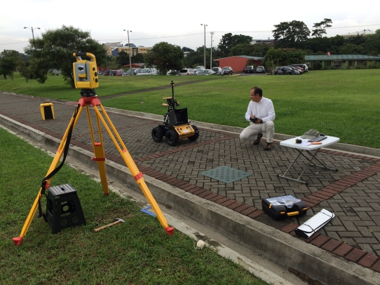
Fig. 1. Clearpath RoboticsTM Husky A200TM rover platform and Trimble® S3 robotic total station used for experimental validation
During each experiment, the rover is commanded to drive on a predefined path at a constant velocity of 3 cm/sec over a paver sidewalk (see Fig. 1), usually a straight segment from 1 to 12 m in length or a 3 m radius arc from 45 to 225 degrees, while a single camera with a real time image acquisition system captures images at 15 fps and stores them in the onboard computer (see Fig. 2). Although the rover’s real time image acquisition system consists of three IEEE-1394 cameras (see Fig. 1)—a 6 mm Grey Point Bumblebee®2 stereo camera, a Grey Point 6 mm Bumblebee® XB3 stereo camera and a 6 mm Basler A601f monocular camera, rigidly attached to the rover by a mast built in its cargo area—only the right camera of the Bumblebee®2 stereo camera was used in all experiments. This camera has an image resolution of 640x480 pixel 2 and a horizontal field of view of 43 degrees. It is located at 77 cm above the ground looking to the left side of the rover tilted downwards 37 degrees. The radial and tangential distortions due to the camera lens are also corrected in real time by the image acquisition system. This image acquisition software was developed under Ubuntu, ROS and the programing language C.
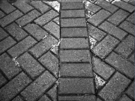
Fig. 2. Image with resolution 640x480 pixel 2 captured by the right camera of the rover’s Bumblebee®2 stereo camera during experiment number 288
Simultaneously, a Trimble® S3 robotic total station (robotic theodolite with a laser range sensor) tracks a prism rigidly attached to the rover and measures its 3D position with high precision (≤ 5 mm) every second (see Fig. 1), where the position and orientation of the local coordinate system of the robotic total station with respect to the planet’s surface model coordinate system at time t 0 is precisely known.
After that, the intensity-difference based monocular visual odometry algorithm is applied to the captured image sequence. Then, the prism trajectory is computed from the rover’s estimated 3D motion. Finally, it is compared with the ground truth prism trajectory delivered by the robotic total station.
All the experiments were performed on an Intel® CoreTM i5 at 3.1 GHz with 12.0 GB RAM. In Table 1 and Table 2, the main experimental results are summarized. The number of observation points N per image was 15906 on average with a standard deviation of 67.74, a minimum of 15775 and a maximum of 15999 observation points. The average number of motion estimation iterations per image was 14.88 with a standard deviation of 1.89, as well as a minimum and maximum of 12.33 and 19.09 iterations, respectively. The processing time per image was 0.06 seconds on average with a standard deviation of 0.006, a minimum of 0.05 and a maximum of 0.08 seconds. The absolute position error was 0.9% of the distance traveled on average with a standard deviation of 0.45%. The minimum and the maximum absolute position error was 0.31% and 2.12%, respectively. These absolute position error results are quite similar to those achieved by known traditional feature based stereo visual odometry algorithms [28, 30, 10, 34], whose absolute position errors of distance traveled are within the range of 0.15% and 2.5%. The tracking was not lost in any of the experiments. Figs. 3, 4, 5 and 6 depict the visual odometry trajectory and the robotic total station trajectory for four different paths driven by the rover, two paths forming arc segments and two paths forming straight segments, respectively.
Table 1 Mean and standard deviation of experimental results
| mean | standard deviation | |
| Observation points per image | 15906 | 67.74 |
| Motion estimation iterations per image | 14.88 | 1.89 |
| Processing time (in second) per image | 0.06 | 0.006 |
| Absolute position error | 0.9% | 0.45% |
Table 2 Minimum and maximum values of experimental results
| min | max | |
| Observation points per image | 15775 | 15999 |
| Motion estimation iterations per image | 12.33 | 19.09 |
| Processing time (in second) per image | 0.05 | 0.08 |
| Absolute position error | 0.31% | 2.12% |
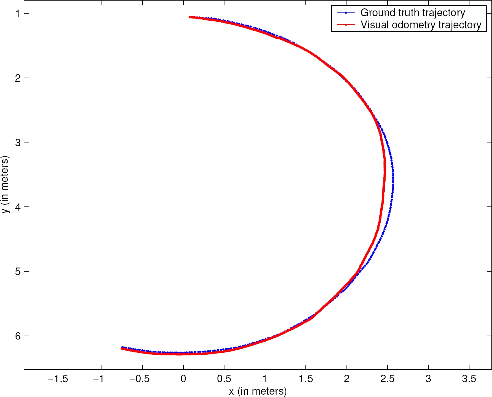
Fig. 3. Trajectory obtained by visual odometry (in red) and corresponding ground truth trajectory (in blue). The rover drove a 3 m radius arc of ∼190 degrees
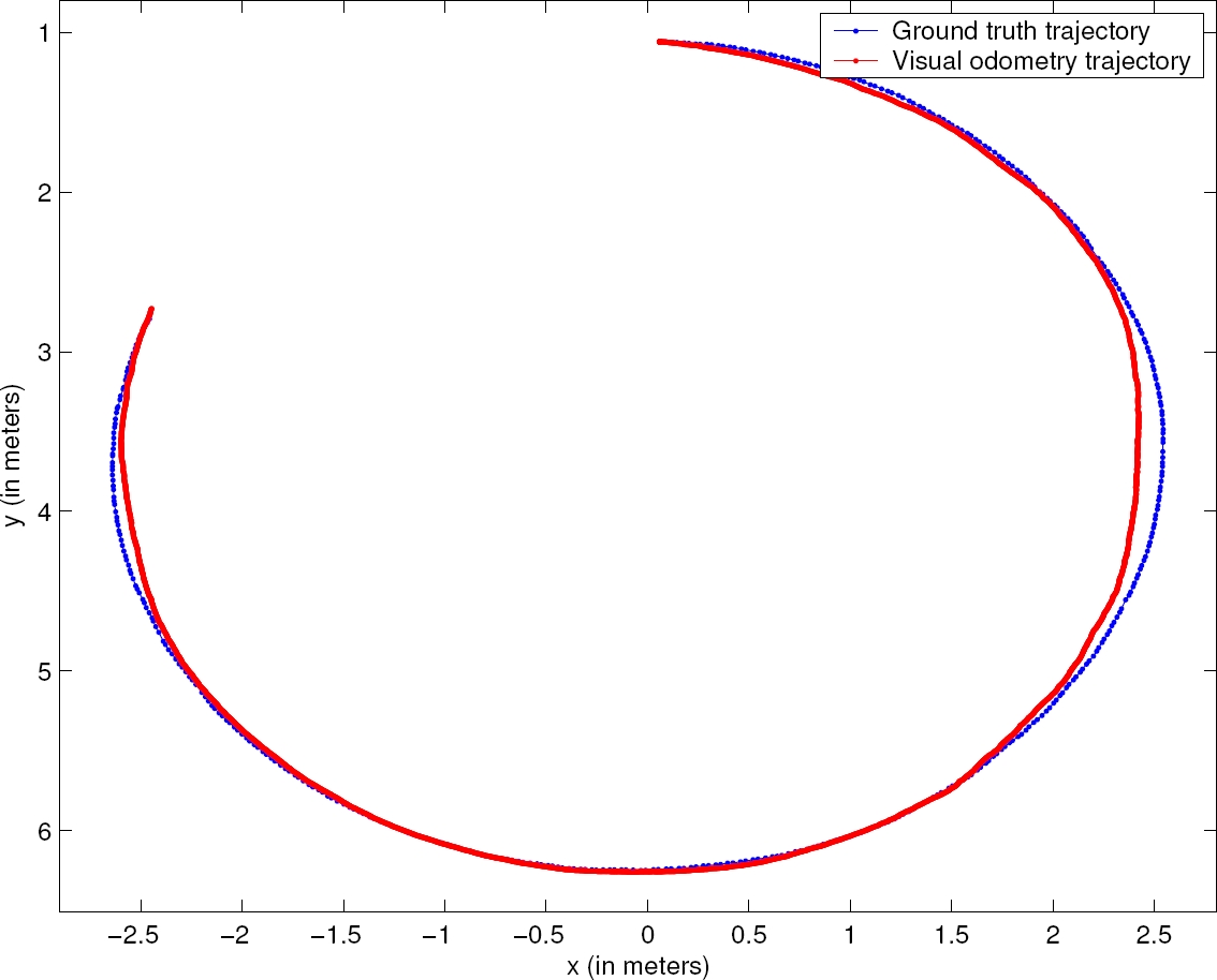
Fig. 4. Trajectory obtained by visual odometry (in red) and corresponding ground truth trajectory (in blue). The rover drove a 3 m radius arc of ∼280 degrees
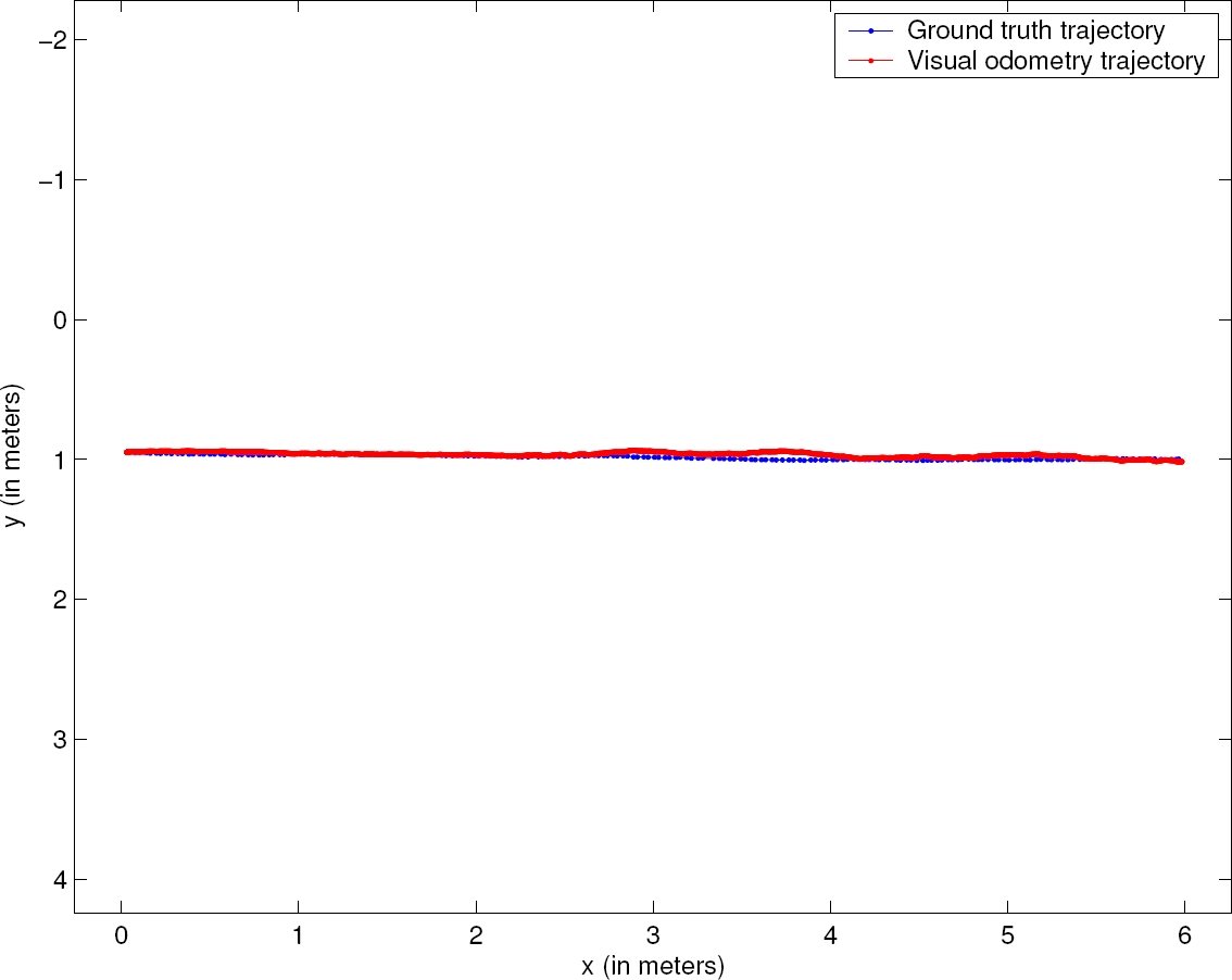
Fig. 5. Trajectory obtained by visual odometry (in red) and corresponding ground truth trajectories (in blue). The rover drove a straight segment of ∼6 m in length
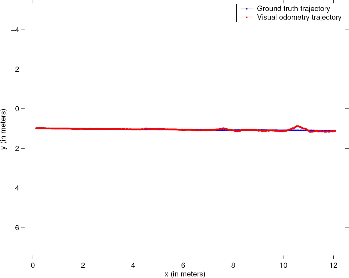
Fig. 6. Trajectory obtained by visual odometry (in red) and corresponding ground truth trajectory (in blue). The rover drove a straight segment of ∼12 m in length
Although our experiments were carried out only on flat terrain along straight lines and gentle arcs at a constant velocity without the presence of shadows, we believe that these results are still relevant because they reveal the potential of the algorithm for obtaining the rover’s position in real outdoors situations, even under severe global illumination changes, in a non-traditional way, without establishing correspondences between features or solving the optical flow as an intermediate step, just directly evaluating the intensity differences between successive frames delivered by a monocular camera.
4 Conclusion
After testing the monocular visual odometry algorithm proposed in [41, 42] in a real rover platform for localization in outdoor sunlit conditions, even under severe global illumination changes, over flat terrain, along straight lines and gentle arcs at a constant velocity, without the presence of shadows, and comparing the results with the corresponding ground truth data, we concluded that the algorithm is able to deliver the rover’s position in average of 0.06 seconds after an image has been captured and with an average absolute position error of 0.9% of distance traveled.
These results are quite similar to those reported in scientific literature for traditional feature based stereo visual odometry algorithms, which were successfully used in real rovers here on Earth and on Mars. Although experiments are still missing over different types of terrain and geometries, particularly over rough terrain, we believe that these results represent an important step towards the validation of the algorithm and that it may be an excellent candidate to be used as an alternative when wheel odometry and traditionally stereo visual odometry have failed. It may also be a great candidate to be merged with other visual odometry algorithms and/or with sensors such as IMUs, laser rangefinders, etc., to improve autonomous navigation of current and future Moon and Mars rovers.
Additionally, since it has the advantage of being able to operate with just a single monocular video camera, which consumes less energy, weighs less and needs less space than a stereo video camera, it might also be especially well-suited for light robots such as entomopters (insect-like robots), where space, weight and power supply are really very limited.
5 Future Work
In the future, the algorithm will be tested over different types of terrain and geometries. Most likely this will require that the precise 3D shape of the terrain is acquired before motion estimation by using a range sensor or stereoscopic camera. We will also make the algorithm robust to shadows by segmenting the shadow regions in the acquired images similar to the proposal in [45] and excluding them from motion estimation.

