


 text new page (beta)
 English (pdf)
 Article in xml format
 Article references
 Send this article by e-mail
 Cited by SciELO
  Similars in
SciELO
Similars in
SciELO 
 Permalink
1 Introduction
A single language spoken in a wide geographical area varies in phonological, grammatical and lexical terms due to historical, cultural, political, social, and geographical reasons. Such linguistic variations are known as dialects [10], which are studied in the field of dialectology and measured quantitatively using methods from dialectometry. Most of such methods are generally based on very few or manually drawn data using language-dependent handcrafted features (e.g. alternations such as mother/mom). These and other drawbacks of current approaches, which are discussed in this paper, make difficult the use of current results for Natural Language Processing (NLP) applications.
In recent research, the Hilbert-Schmidt independence criterion test (HSIC) [3] has proven to be effective for measuring the spatial autocorrelation of different types of linguistic variables. In addition, HSIC is non-parametric, almost free of assumptions on the data, and robust against non-linearities in the geographical and linguistic variables. The aim of this work is to propose a method for aggregating the results of the HSIC test on a relatively large number of linguistic variables (thousands) preserving the main properties of HSIC. The goal of such method is to provide statistical evidence of the existence of dialectal boundaries. We named these boundaries “dialectones” following the “ecotone” ecology concept (i.e. a boundary of ecological change) and borrowed ideas from that field to provide a comprehensive definition.
The paper is organized as follows. In Section 2, we present a critical view of some of the issues of current practices in dialectometry, which are addressed in some way in this paper. In addition, we provide a parallel between the proposed dialectone and ecotone concepts. In Section 3, we present proposed method and its motivations. In Section 4, we test the proposed method using Twitter data collected in Colombia and the results were compared against previous dialectal studies in that country. In Section 5, we compare the methodological key factors of the proposed method applied to the Colombian data against a recent study (2016) [6] in the United States, which we consider representative of the state of the art. Finally, in Section 6 we provide some concluding remarks.
2 Background
2.1 A Critical View of Current Paradigms in Dialectometry
The usual pipeline in classical dialectometry to obtain dialectal regions basically consists in 1) selecting a set of linguistic variables that has regional variation; 2) selecting a set of geographic locations for collecting data to instantiate the selected variables; 3) building a square matrix of linguistic distances (or similarities) between pairs of locations using some mathematical measure; 4) organizing the regions into groups using clustering techniques, usually combined with dimensionality reduction techniques (e.g. Principal Component Analysis, PCA); and 5) visualizing the found groups as regions in a geographical map. This methodology has several known issues that have been noted the in the recent literature [12, 4, 13]. These and other issues are discussed bellow.
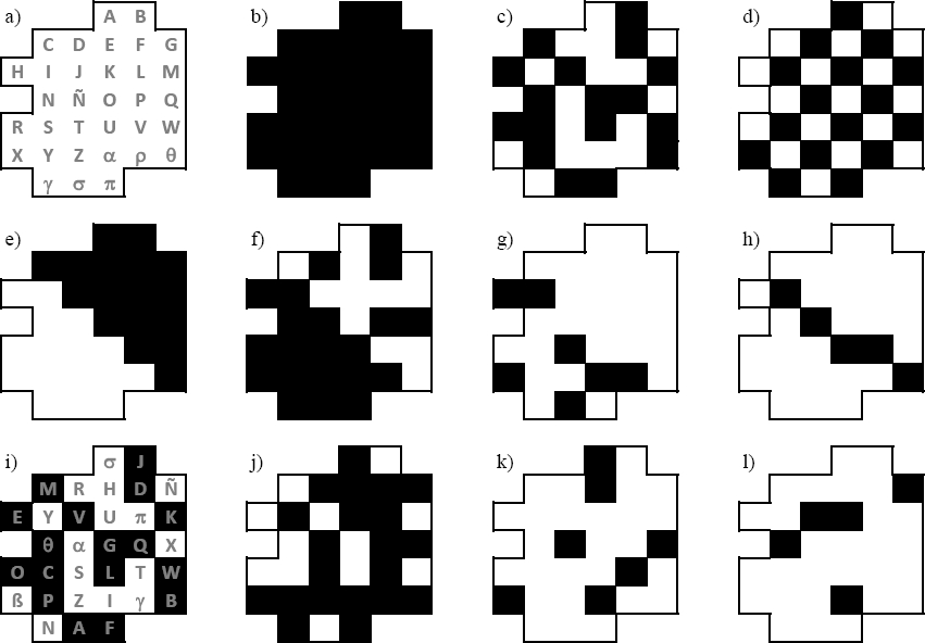
Ignore geographical coordinates in the analysis. Classical dialectometry ignores the coordinates of the locations when building the distance and similarity matrices and only takes them back in the last step for the visualization. However, it is widely known in geographical, ecological and social sciences, among others, that the variables to be study linked to geographical locations reveal patterns impossible to discover if the two-dimensional space where the data was collected is ignored. To illustrate that situation, we propose a didactic resource borrowed from spatial autocorrelation. Let us consider a hypothetical island divided into 33 counties named after letters as shown in Figure 1a. Now, on each county, we depict a binary linguistic variable (e.g. a binary alternation). The maps in the first row in Figure 1 show patterns lacking any regional factor, i.e. absence (a), ubiquity (b), random (c) and uniform distribution (d). Unlike that, the patterns in the second row show a clear division between the north-east and the south-west of the island. These patterns combine absence\ubiquity (e), ubiquity\random (f), random\absence (g), and a frontier (h). The aggregated information of these 4 variables reinforces the evidence of the existence of 2 dialects in the island. To illustrate our point, we shuffled the locations of the island and showed the same data from the second row into the third row. Clearly, the regional patterns in the data disappear and the variables become indistinguishable from randomness. However, any analysis that disregards the geographical coordinates would yield the same results for the second and third rows.
Assumption a priori of the existence of dialects. As Grieve et al. [4] noticed, most of the dialectometry approaches serve to confirm the assumptions of the researcher rather than proving the existence (or not) of dialectic regions. In the first step of the above-mentioned pipeline process, the researcher selects linguistic variables (usually alternations, e.g. mother-mom) that produce dialectic regions where these variables reveal patterns. However, if elsewhere in the studied zone there is an actual dialect, but none of the selected variables changes in that region, then that dialect remains hidden in the analysis.
The lack of statistical evidence. Grieve et al. also noticed that most of the dialectometry analyses are performed using methods weak against random noise in the data. That is distance and similarity measures that do not provide information about the significance of the scores that they produce. Thus, there is no way to distinguish which revealed patterns are produced by a dialectal region or by randomness. Recently, the use of statistical tests for spatial autocorrelation, such as Moran’s I, Mantel test and others, are being used in dialectometry [4, 6]. However, these statistical tests are being used only for variable selection. In this paper, in addition to these kinds of tests, we aim to provide a statistical test for the further steps of aggregation of the variables.
The need of parameters [12]. Clustering plays an important role in classical dialectometry. However, in practice, all clustering methods require adjusting parameters, which in one extreme of their spectrum group all instances in a single group, and in the other make a group of each instance. Only at some intermediate values of the parameters, the researcher recognizes the expected dialectal regions.
The previous issues indicate that classical dialectometry is more a qualitative tool for assisting the researcher rather than a data discovery tool. In that scenario, these methods are not suitable for NLP applications where prior dialectal information is not available and raw data is the only information source.
2.2 Ecotone and Dialectone
In ecology, for more than a hundred years, researchers have been searching for the area that divides adjacent ecological communities, which they call ecotone. Researchers in dialectometry, for their part, look for the areas that divide dialects. The idea of associating the ecotones with linguistics was first suggested in 2013 by Luebbering [9]. The boundaries of the dialectal areas could be called dialectone, by extension of the first concept. A definition for ecotone that is more inclusive than many others is that of Holland et al. [5]: “Ecotones are zones of transition between ecological systems, having a set of characteristics uniquely defined by space and time scales and by the strength of interactions between adjacent ecological systems”. The above statement comes from Hufkens et al. [7], who compared the definition of Holland et al., to those reviewed between 1996 and 2006. They argue the concept of ecotone must have semantic uniformity. In addition to comparing the definitions, they listed the techniques used to identify and describe ecotones: moving-split window, ordination, sigmoid wave curve fitting, wavelets, edge-detection filters, clustering, fuzzy logic and wombling [17].
Given the above and based on the definitions shown by Hufkens et al. [7], we could define dialectone as: “a zone of transition between adjacent dialects, having a set of characteristics uniquely defined by space and time scales and by the strength of interactions between adjacent dialects”. Thus, the dialectones could be identified and described by means of some techniques applied to the ecotones. This implies a change of paradigm in dialectometry because it stops looking for regions using grouping, parameters, and subjectivity in the interpretation, to look for linguistic change borders with statistical methods without (or with few) parameters and giving evidence of the existence of the borders.
Some characteristics that describe the ecotone concept can be extrapolated to dialectone. In an ecotone there is richness, abundance and occurrence of unique species [14, 8]. The same can happen in a dialectone, where there can be a variety of words for the same reference (wealth and abundance) and unique words (regionalisms). Another characteristic of ecotones is that there is active interaction between two or more ecosystems. This interaction modifies the original ecotone and makes it acquire new properties, which were not present in any of the ecosystems involved [15, 8]. The above also applies to a dialectone. The interaction between speakers of two different dialects, in the same area unknown to them, means that they must create words to communicate and describe this area. Words that will only belong to this area and that are not part of the vocabulary of any of the dialects involved. Another characteristic of ecotones is that their location and coverage evolve over time with local or global consequences [16, 7]. A dialectone could have this characteristic, since the speakers move to other areas taking their lexicon with them.
3 Method
The proposed method for detecting dialectones in a geographical region is detailed in the following steps (the motivation for each step is discussed in the further paragraphs).
Determine a region for dialectal study and select a set of representative locations.
Collect a corpus of texts (e.g. tweets) for each location.
Let L be a subset of locations with corpus larger than α tokens.
Collect longitude and latitude coordinates for the locations in L.
For each word w in the corpora do:
Collect a vector of relative F w of frequencies indexed by locations in L.
Compute the spatial autocorrelation between F w and the geographical coordinates of L using the HSIC test [3].
Get the set of words W from the top-β words with the highest values of the HSIC statistic and satisfying significance p < 0.05.
Compute a Voronoi’s tessellation for the L locations.
For each pair of neighbor locations a and b in L do:
For location a get a vector of frequencies F a (from F w vectors with relative frequencies by location) indexed by the words in W .
Ditto for location b.
Determine among a and b, the location with the smallest number of non-zero relative frequencies in F a and F b . Let w be set of words with non-zero relative frequencies in that location, and n the size of w.
Compute the Wilcoxon signed rank test between the relative frequencies from the n pairs indexed by w in F a and F b vectors.
Normalize to the [0, 1] interval the value of the Wilcoxon statistic T by dividing it by n(n + 1)/2.
If the resulting statistical significance is p < 0.05, then a dialectone boundary was found. So, draw in the map a boundary line between locations a and b by coding the value of the Wilcoxon statistic in the line width (thicker for larger values).
Return the map of dialectones for the region with statistical significance p < 0.05 for parameters α (minimum size for the corpus of each location) and β (the number of top regional features tested).
In step 1, the researcher should decide the type of location (e.g. urban, rural), density and coverage according to their goals. Similarly, in step 2, the source of linguistic information should be determined. Step 3, is necessary to keep control of the effect of the size of location corpora. If the corpus of a particular location is too small, then the occurrences of the words in the W set can be too small to find a significant pattern. Thus, parameter α controls this factor. In our experiments with the data described in subsection 4.1, we used α = 50, 000 reducing the initial number of locations from 231 to 160.
In step 5, the spatial correlation of every vocabulary word in the corpus is computed to identify their degree of regionalism. For that, the Hilbert-Schmidt independence criterion (HSIC) has been used following the recent findings of Nguyen & Eisenstein (2017) [13], who showed that HSIC outperformed other known spatial autocorrelation tests (i.e. Moran’s I, Join Count Analysis, and the Mantel test) in the task of detecting geographical language variation. In addition, the HSIC test has the advantage of being non-parametric. In our experiments, we used a Gaussian kernel and the implementation provided by the authors1.
The other aspect to determine at this point is the representation used for each word. First, we considered the alternative of using frequencies or rankings of the words as entries on the F w vectors. Another possible decision is the alternative of using raw frequencies and rankings or using “relative” versions divided by the maximum word frequency in the corpus for the location or by the location vocabulary size, respectively. The motivation for this is to keep control of the imbalance in corpus size between locations by using the “relative” versions.
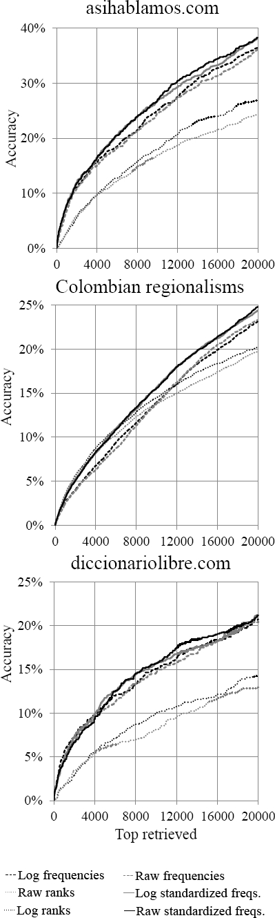
Finally, motivated by the Zipf’s law [18], which states that log(frequency) ≈ −k · log(ranking), we considered the alternative of linearizing the data by applying the logarithm function. To evaluate the previous options, we collected 3 lists of regional words for the Colombian Spanish: AsiHablamos.com2, DiccionarioLibre.com3 and the forthcoming Dictionary of Colombian Regionalisms4.
The values of the HSIC statistic were computed for each of the proposed alternatives of representation using the 20,000-top frequent words in the corpus. Next, the words on each resulting list were sorted decreasingly (most regional words first) by the HSIC statistic. Lastly, each list was compared against the 3 dictionaries (see Figure 2) reporting the percentage of words from the dictionaries as words from the sorted lists are retrieved. Results in Figure 2 show consistently that the best representation is the use of relative frequencies (continuous black line).
Once, the vocabulary words from the corpus are ranked by their regionalism degree, the list contains true regional words only until some ranking β, where the regional character of the words fade out (step 6).
Manually reviewing the HSIC scores using the data from subsection 4.1, we determined that β = 20, 000 is a convenient threshold. In addition, the regional words must be filtered by statistical significance using p-values computed performing permutation tests with 500 samples. Filtering by the customary p-value of p < 0.05, 15,993 words remained in the W set out of the initial 20,000 words.
In step 7, the geographical locations of the boundaries between each pair of neighbor locations are determined with the Voronoi’s tessellation. Next, each one of these boundaries will be statistically tested (step 8) with the Wilcoxon rank test under the null hypothesis that both locations have no-dialectal variation.
Note that the Wilcoxon and HSIC tests are non-parametric, making the proposed method non-parametric too (α and β can be considered as hyper-parameters of the method). When comparing 2 neighbor locations with a considerable corpus imbalance, say |a| ≪ |b|, the vector F a has considerably more zero entries than in F b . That situation can produce a size effect in the Wilcoxon test. To lessen this, one can remove all zero entries from the test (common vocabulary) or the zero entries of the location with the lower number of zero entries (smallest vocabulary).
In Figure 3, we analyze (using the same Colombian data) the behavior of the normalized Wilcoxon T statistic as the corpus imbalance varies for 3 scenarios (vocabulary proportion is |a|/|b|). At right, all words in W were used in the test showing a clear dependence of the variables. A similar pattern occurs in the figure at center (common vocabulary). Clearly, the best alternative is smallest vocabulary showing the better independence between T and the imbalance factor.

4 Experimental Validations
4.1 Data
Following the current trend of using Twitter data for dialectal analysis [2], we collected a large corpus of geolocated tweets in Spanish from Colombia. Firstly, 237 cities were selected having at least 10,000 inhabitants according to the 2005 Colombian Census5 and by removing small cities that were mostly overlapped by a radius of 15 miles around cities with more than 100,000 inhabitants or 7 miles for the remaining cities. Next, we collected tweets between the years 2009 to 2016. The resulting corpus contains approximately 28 million tweets produced by 1.5 million users making a total of 291 million of tokens after removing hashtags, usertags, and URLs. As reference, the Colombian population is estimated for the year 2017 in approximately 48 million. Therefore, the corpus roughly comprises the 3% of the population. The geographical coordinates for each city were obtained from Google Maps. Finally, we removed any non-alphabetical tokens, acronyms, words with more than 3 repeated letters (e.g. holaaaaaa) and proper nouns, which were detected using occurrences of words with initial capital letters collected throughout the entire corpus.
4.2 Results
Figure 4 shows a map with the dialectones found with the collected data. The dialectones are represented in the edge line of each pair of locations. The dialectone width shows the value of the Wilcoxon T test Correlation. We only draw dialectones with statistical significance (p < 0.05), and represent possible influence of corpus imbalance by dotted lines (rank correlations between 0 and 0.3, see Figure 3). For qualitative comparison purposes, Figure 5 shows dialectones (left) and 2 maps that represent Colombian dialectal regions obtained using classical dialectometry methods.
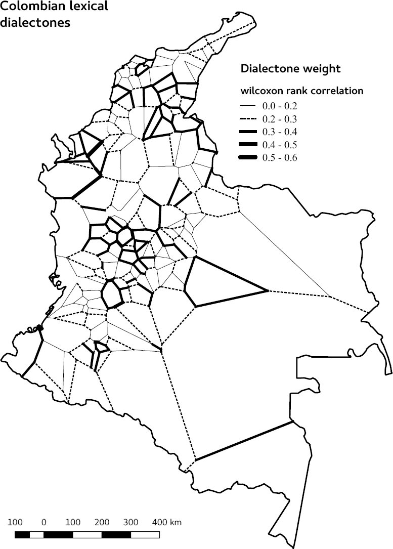
Fig. 4. Found dialectones in Colombia using Twitter data (2010-2016) with p < 0.05, α = 50, 000 and β = 20, 000. Dotted lines (ranges between 0 and 0.3) represents rank correlations which can be affected by the difference in corpora size

Fig. 5. Map of dialectones (left) and two dialectal distributions: Dialectometry Clustering (center) and traditional dialectology isogloss (right). Cluster map obtained by a matrix of similarities and differences based on lexical data of 200 random maps of the ALEC [1]. The isogloss map is the dialectal proposal of the Department of Dialectology of the Caro y Cuervo Institute presented in [11]. The thick diagonal line drawn by us on each map points to the most important zone of similarity between the three maps
4.3 Discussion
Unfortunately, there is not a “gold standard” to evaluate our results against it. The most accepted dialect proposal on Colombian Spanish is based on data with more than 40 years and that were collected and processed with different methodologies than ours. However for qualitative comparison, in Figure 5 we present our map next to two dialectal proposals based on the ALEC [1]. We draw in each of them a thick diagonal line that indicates the area that in our opinion is analogous to the three maps. That area corresponds to the most important dialectal division of the dialects of Colombian Spanish: Andean and Costeño. The most noticeable visual difference between the dialectones and the other two representations is perhaps that with the traditional methods a continuous border is observed, while the frontier marked by the dialectones is discontinuous. However, it can be seen in Figure 4 that the dialectones with the greatest Wilcoxon’s correlation are located close to the line we draw in Figure 5. Therefore, the statistical evidence supports the idea that in that area exists a dialectal border.
5 Related Work
Though the research in dialectometrics is vast, we consider the recent work of Huang et al. [6] representative of the state of the art. Table 1 contains a comparison of the key factors between that work and the approach presented in this paper. Although both works address different languages and countries considerably different in size, they are comparable in the goals and the density of the data (per capita), which is approximately in a 4:1 ratio of theirs vs. ours.
Table 1. Comparison of the work of Huang et al. 2016 against this paper
| Aspect | Huang et al. 2016 / This paper |
|---|---|
| Geographical region | United States / Colombia |
| Corpus source | Twitter 2013-2014/ Twitter 2010-2016 |
| Corpus size | 7.8 billion words / 291 million words |
| Number of locations | 3,111 counties / 237 cities filtered to 160 |
| Universe of lexical features | 211 predefined lexical alternations / ∼ 1 million (the entire corpus vocabulary) |
| Feature selection method | Heuristics and Moran’s I p < 0.001 / HSIC statistic and p < 0.05 |
| Number of selected features | 38 / Top-15,993 words using HSIC statistic |
| Values of the features | Mean variant preference (MVP) / Normalized word frequencies |
| Handle of noise | Smoothing with a Gaussian kernel / statistical significance |
| Dimensionality reduction | Principal component analysis (PCA) / none |
| Comparison of locations | 2D visual clustering / Wilcoxon’s signed rank test |
| Map visualization | Counties areas filled with colors / Line thinkness in a Voronoi tessellation |
| Type of detection | Dialectal regions / Dialectal boundaries (i.e. diatectones) |
| Statistical significance of the results | none / p < 0.05 |
The first important difference is the method for selecting the features to be analyzed. While they start with a manually collected set of 211 alternations (filtered to 38 using Moran’s I spatial autocorrelation), we considered the entire vocabulary of the corpus and filtered out to approximately 15,000 words, which happen to be significant using HSIC spatial autocorrelation. This is an important methodological difference because using a small set of predefined features they make use only of a very small portion of the corpus. In contrast, filtering the entire vocabulary throughout the entire corpus provides a larger set of significant unbiased features. Moreover, as Nguyen & Eisenstein showed [13], the HSIC test is a better alternative for Moran’s I when using linguistic variables.
Regarding the values of the features, both approaches (mean variant preference vs. normalized word frequencies) provides a mechanism for controlling the effect of corpus imbalance for pairwise location comparison. However, our selection of using normalized frequencies is supported by an extrinsic evaluation against dictionaries of regionalisms build by professional lexicographers and crowdsourcing. Moreover, unlike alternations, frequencies are language independent.
Another important difference is the method for handling noise and locations with missing or very few data. The approach of using smoothing seeks to reduce abrupt variations in the data by replacing the original data by an aggregation of the data itself and that of its neighbors.
Instead of making modifications to the data to soften outliers or complete missing data, we propose statistical tests to discard cases when abrupt changes could produce a false pattern due to randomness and when the lack of data makes the result non-significant.
Finally, though the visualization of dialectones is harder to interpret, it only shows the dialectal boundaries that can be inferred with confidence from the data. Again, in our opinion processes such as PCA and clustering, which improve visualization, modifies the original data and introduce parameters, whose variation produce important changes in the visual outcome.
6 Conclusions
We introduced the concept of “dialectone”, a geographical boundary where 2 dialects of a language show a significant variation. The proposed method for detecting dialectones is non-parametric and language independent, overcoming several methodological issues of classic dialectometry, particularly the lack of statistical evidence of the existence of dialects. Nevertheless, the proposed method for detecting dialectones is limited to lexical evidence. Finally, the dialectones have the potential of being used in NLP applications sensitive to dialectal variations by providing an unbiased measure of language change in a geographical region.

