


 text new page (beta)
 English (pdf)
 Article in xml format
 Article references
 Send this article by e-mail
 Cited by SciELO
  Similars in
SciELO
Similars in
SciELO 
 Permalink
1 Introduction
Wind power generation has become a critical contributor to the electrical supply systems in many countries around the world. We can cite some nations with high wind penetration in their electricity generation mix (as a percentage of total production in 2016) like Denmark (36,8%), Ireland (27%), Portugal (24,7%), Spain (19%) or Germany (16%) [39]. This penetration, already relevant, will see a steep increase in the next few years due to the renewable push that will happen when the Paris climate agreements [37] are implemented in national policies.
IT is clear that renewable generation will be the primary source in the decarbonized future, at 100% or close to that number, and the load balancing in the Grid will have to cope with the intermittency and load characteristics of this generation sources. It is clear that the future will be renewable.
In this context, developing more reliable techniques for the integration of wind power is critical for the electrical Grid stability, and forecasting the energy generation output is a key task. Wind energy forecasting has not only value for its contribution to the system stability as it has a strong potential for savings in the overall system. But it has also been established that a small increase of 10% in the quality of prediction would be able to generate savings of 140 million US$ in the United States alone [20].
Many methods have been designed for wind prediction, which belongs to two main groups: meteorological methods based on weather prediction and methods (also categorized as statistical) based exclusively on Time Series data.
Wind time series are complex and difficult to forecast, and many methods have been tried, from the easy and accurate short-term persistence, or some adaptations of this method [28], or the whole family of linear time series models (AR, ARMA, ARIMA, etc.), some non-linear statistical methods, and finally the Artificial Intelligence (AI) methods. In this paper, the focus will be in the last category, analysing the use of AI methods, with an emphasis in machine learning first in neural networks and second in the nascent deep learning approaches.
2 Wind Energy Generation Forecasting Task
Energy in the turbines is generated from the kinetic energy of wind. The action of wind moves the blades and generates a rotational effect which produces electricity (by the Faraday law). In the field wind turbines are usually grouped in wind parks that can range from a few turbines up to hundreds to leverage areas where the wind is steady and strong over the whole year. The power generated by a wind turbine (see equation (1)) is directly dependent on the swept area of the Blade (A), or on the Air density (ρ), but mainly on the airspeed (v), (cubic in the formula), and finally Time (t) is linearly dependent in the Energy (E) Formula, where Power does not depend on time:
In figure 1 a graphical representation of the transformation of wind speed into power can be observed. The red-coloured points are tuples of energy generated with wind speed (in 10 min periods). In this graph, the points concentrated along the original theoretical power curve (each turbine has its own). Additionally, it can be seen the existence of two relevant points: (a) the cut-in which defines the speed at which the turbine starts generating energy and, (b) the cut-off which is the threshold where there is no additional power generated (it is quite usual that this point triggers safety mechanisms to avoid the blades to be damaged by strong winds).

There is some discussion about if it is better to forecast wind speed or power generated, with no consensus on this issue. Some sources like the Anemos report [10] show a preference in power forecasting based on a filtering effect that will be caused by using the power function from the wind. Generally, it is recommended to develop a power function for every real turbine from real observations [34]. This can help to reduce the error since it is estimated that the differences between the wind power function calculated experimentally by the company maker and the real turbine can be as high as 20% [3]. Whatever the objective is (wind or power), in the end, the ability to understand and learn the wind patterns is critical to obtain good forecasts.
Other techniques add post-processing procedu-res to the wind forecast data like Kalman Filters that smooth the data in the transformation from wind to power. This approach is well defined in the literature as well and found in many experiments, like [25].
Looking at the characteristics of the Power curve (see example in Fig. 1), the wind speed forecasting errors can be amplified in the high-slope, and the errors in the cut-in and cut-off areas are dampened. In this sense, the recommendation is to use power forecasting and use specific power curves for the turbines or even develop aggregate models for wind parks, and this will lead to more accurate results [40].
In the commercial applications, the final ob-jective is to find the best possible power prediction, using all the tools available, and to perform this, independently of the approach, it is required to discover the internal patterns of the wind for a particular geographic location.
Even in approaches with complex post-processing transformations or statistical inference, some insight of the mechanics of the wind generation and how this forecast transforms into energy is required. We can segment the forecasting problem into two: the forecasting of wind and the transformation of wind speed into power.
The power conversion function ties wind and Power, and this work analyzes how different forecasting models based on Machine Learning approaches can learn the inner structure of the wind time series to increase the performance of the forecasting exercise.
3 Nature of Wind Time Series
Wind turbines are provided with hundreds of sensors that offer information in real time, generating a stream of data to be analyzed, like the energy generated, or the performance of the internal engines and mechanisms and meteorological data about the environment (wind speed, temperature, pressure, etc.). Different applications analyze all this data, and one of them is the prediction of the energy output.
For this task, the information of the sensors is converted into time series with readings every 5 to 10 minutes. Typically, a wind time series will be a set of observations of several years long containing several variables (wind speed, temperature, humidity, pressure, wind direction, density, etc.). In Fig. 2, it can be seen the wind speed dimension of a turbine over six years of data.
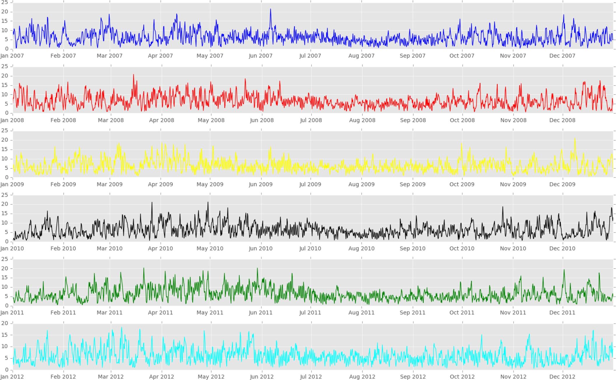
Fig. 2. Wind speed time series in site located in Techado, vertical axis wind speed in m/s, horizontal axis time, New Mexico. NREL Dataset [7]
Wind is a natural phenomenon that is created by various forces applied to the atmosphere at the same time, namely: the pressure gradient force, the frictional force, the Coriolis force and the gravitational force. For the energy forecast task in wind turbines, only winds close to the surface are studied, and those are impacted by the frictional force, which will depend on the specific orography of the site [16]. It is well-known that wind may vary in two locations not far away. It can be seen in a wind park the different speed of the blades in similar turbines or some turbines idle (no wind) while some others are turning, this is an empirical test of the wind variation due to orography factors.
But not only orography is relevant for the wind formation. The earth science has already stated that wind is the combination of periodical phenomena like day/night or summer/winter, a result of low/ high-pressure variations and all of them combined with temperature, air density and pressure. The combination of all these factors is of high complexity and the result, over time, is the wind as we know it.
For this reason, it is quite usual that in a wind time series all these factors are overlapped (a storm in summer at night from the north), and extracting each factor is of high complexity (if possible at all).
A wind time series will be a time-stamped sequence of several measures that can be related to wind. The dimensions are usually (some or most of them); wind power (MW ), wind direction (degrees), air pressure (P a), wind speed (m/s), temperature (C or K), air density (kg/m 3), relative humidity (%). All these observations can be generated at different heights (floor, hub height, half height). As the wind at 100 meters high (hub turbine height) is the one that moves the blades, it is probably the measure with the highest relevance, while wind direction is important to understand how the dominant winds might impact wind patterns and intensity. In Fig. 3 a summary of one-year data from the Sotavento wind park is shown in the wind rose, the dominance of E/NE and W/SW winds is clear on this site.

Fig. 3. Wind direction dimension in one year of time series measurements in the Sotavento Park located in Galicia, Spain 2016 [5]
3.1 Non-Stationarity of Wind Time Series
Stationarity in a time series is understood as the property where the statistical characteristics such as mean, variance, autocorrelation, etc. are all constant over time, or repeat over time in some sequences (seasonal, day/night,...).
There are several tests widely used to analyze the stationarity of a time series. The Dick-Füller (ADF) test (and its evolution the augmented ADF) are the most common [6]. The ADF looks for a unit root in a time series sample. A unit root is a statistical feature that determines randomness in the series. The ADF Tests sets up a hypothesis that there is a unit root. The more negative is the result, the higher the rejection of the hypothesis, and the probability of the time series being non-stationary increases.
In Table 1 an example of ADF test is shown where the negative ADF shows clear non-stationarity in two sample turbines in the NREL dataset.
Table 1 ADF test on two NREL dataset sites (using ADF statsmodel)
| Offshore New Orleans | Edgeley North Dakota |
|---|---|
| turbine: 3007 | turbine: 112500 |
| latitude: 28.580738 | latitude 46.292343 |
| longitude -90.734619 | longitude -98.736877 |
| ADF Statistic: -31.418378 | ADF Statistic: -44.676385 |
| p-value: 0.000000 | p-value: 0.000000 |
| Critical Values: | Critical Values: |
| 1%: -3.430 | 1%: -3.430 |
| 5%: -2.862 | 5%: -2.862 |
| 10%: -2.567 | 10%: -2.567 |
When this test is applied to a time series, if the result is positive it will show stationarity, but if the result is negative then the hypothesis of non-stationarity is confirmed and then the series is considered as non-stationary. Wind time series are most of the time non-stationary, but in some locations (steady winds or very clear seasonal trends) it can lead to some stationarity results.
3.2 Non-Linearity of Wind Time Series
Linearity is another relevant property to be found in the wind time series. Linearity will allow the use of linear forecasting methods and non-linearity needs of more complex methods (non-linear) have to be used to obtain accurate predictions.
The validation of linearity in a time series is not an easy and straightforward task. The surrogate data method, described by Theiler in [36] is a powerful tool to validate linearity. This test applied to wind time series shows that linearity can be found in some wind datasets but not in all of them, and correlations are found in differenced data [8].
If the wind is nonlinear, how can linear models be used for forecasting? The answer lies in the fact that the wind series contains structures that might be linear.
The best forecasting methods will extract this information (learn) the shape of these internal structures to produce more accurate results.
4 Review Methodology
The possibility to use Machine Learning (ML) to analyze historical and new data, to support the physical control operations, and allow decision making based on information extracted from data is having an immense impact in many fields. In particular, the first of these algorithms in wind forecasting started as early as 1990, but its use was not widespread due to lack of conclusive results and the high computing cost. With the recent developments in Deep Learning (DL) new approaches based on deeper architectures are appearing in the literature, and this new interest is generating some experiments that show a good fit for the task.
In this article will review the state-of-the-art of NN and DL applied to wind time series, focusing especially on the most recent developments in the area.
To classify these architectures is a complex task (see Fig. 4) as there are many variations and refinements on top of the primary network categories. To obtain some clarity an effort to classify the approaches in 3 main classes has been made, being those: n-layers Perceptron (MLP), Convolutional networks (CNN) and Recurrent Networks (RNN).
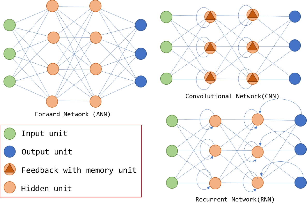
4.1 Perceptron with n-layers (MLP)
The most straightforward architecture of Neural Network has been called Perceptron or Feed Forward Network (see Fig. 4). In this architecture, each layer of the network only has forward connections with the subsequent layer. The Perceptron definition was described in the seminal book from Minsky and Papert Perceptrons [26], but its first implementations come from some years earlier. The basis of the Perceptron is to mimic (loosely) the behavior of the natural neuron and its connections. A signal or data goes into the input layer, then is treated by the hidden layers and the result is made available at the output.
The goal of an MLP network is to approximate some function f*, when there are multiple layers, each layer is a function of the function:
in this three-layer example each function is a layer in the network (one, two, three). This number defines the depth of the model, being the last layer of the output layer.
Neural Networks have on each neuron an activation function that acts on the inputs received and generates an output, plus a backpropagation algorithm that optimizes the weights on each connection in a process to find the optimal combination for the output. Neural networks are non-linear, and this characteristic allows them to produce better results than linear models on wind data time series.
4.2 Convolutional Networks (CNN)
These networks (see Fig. 4) are specialized in processing matrix data (like images, or time series). The name comes from the convolution operation which is a known operation in Calculus which is seen as an integral transformation (see equation (2)):
or for finite matrices the use of Summation instead of integrals:
Convolutional networks can work in large image matrices and extract features from small areas of the matrix, areas that could have relevant features for the task. For instance, in a classification task of birds, the most relevant feature will be the beak and the pixels around the beak will be the convoluted feature of the main image.
In time series, the convolutional networks would be able to identify short intervals of the time series that could bring relevant information to the prediction task. It could be that some patterns in the wind series are relevant for the future behavior of wind.
4.3 Recurrent Networks (RNN)
Recurrent networks (see Fig. 4) are designed to process sequential data, and the most important idea on this construction is sharing parameters between the different layers and neurons, generating cycles in the graph sequence of the network. In this sense, RNN can have memory and use information that is far away in time. An example of RNN is the Long Short-Term Memory (LSTM) which combine convolution over a sequence, being the output of a function of a small part of the input sequence.
In an RNN each output is a function of the previous elements. In a way, RNN work in cycles as the values in a specific step will influence its value in future steps. RNN come with many refinements, like recursive, Elman, Bi-directional and many more. RNN networks have the potential to learn from patterns in the time series to predict the future, and this learning, thanks to the ability to use history in the process, can be used for forecasting purposes.
CNN and RNN have potential features that could help to predict future from learning from the past. The challenge of this application has to do with the internal structure of wind time series. We know they are non-linear and non-stationary, but is in the time series some hidden pattern that tells the behavior of this meteorological phenomena in the future? Is deep learning able to discover this pattern? Which is the most efficient deep learning architecture to use this patterns in the wind speed forecast task?
5 Review of Experiments
A set of relevant works have been selected from the literature and analyzed and presented in tabular form in Table 3.
Table 2 Review summary of different methods
| T | Author | Data | Architectures | Results | Comments |
|---|---|---|---|---|---|
| MLP | (Liu 2016) [23] | 7 farms with real + meteo data | DNN, SVM, ANN | Best, MAE 6h = 12 | Rolling structure of algorithms |
| MLP | (Tao 2014) [35] | wind turbine Mongolia 10 minutes | DBF 3 layers 100/200/300 neurons | Stable results 6-24 hours ahead | Better performance for mid-term forecast |
| MLP | (Pormousavi 2008) [12] | Several sets wind speed 2.5s | ANN 2 layers integrated with Markov | 15% improvement MAPE with MC | Probabilistic approach for very short term prediction |
| MLP | (Hossain 2012) [11] | Rockhampton Solar and wind data | ANN with 11 variables | non-qualified results | integration Solar/Wind - extensive use of exogenous variables |
| MLP | (Ranganayaki 2016) [30] | Two year data observations from 2 wind park sits (India) | ANN ensemble (4 variants) | times 2 to 10 improvement over previous experiments in MSE for short term prediction | Develops a methodology for the calculation of hidden nodes |
| MP | (Sapronova 2016) [32] | NA 2.5 s | ANN, DL architecture | 20/25% improvement over ANN (MAE or RMSE) | Very short term prediction, architecture not specified in detail |
| MLP | (Shi 2012) [33] | NREL North Dakota 1 to 7 steps | ANN+ARIMA+SVM hybrid | Only 3% improvement hybrid over single method | Hybrid does not always generate better performance |
| MLP | (Liu 2013) [22] | 25 days wind data Wind Farm Qinghai China | ANN-Wavelet-ARIMA hybrid | Wavelet + ANN (BFGS) best model | Hybrid is marginally better but more costly |
| MLP | (Li 2010) [21] | North Dakota sites, 1 year hourly sampled | 3 ANN architectures | Best model depends on data | There is not a ’best’ model |
| CNN | (Diaz 2015) [4] | Meteo Data, 1 farm and Areas in Spain | CNN and NN | MAE 5% than SVR algorithm | Experimental algorithms with promising results, need further experimentation |
| CNN | (Wang 2017) [38] | one year data from 2 wind farms in China | CNN DL Architecture | 20% up to 600% improvement in some time frames | Decomposition of time series in signals of different frequency |
| RNN | (Ghaderi 2017) [9] | 57 locations meteo data | RNN and LSTM architectures | RNN best results | Architectures manage to obtain good results in one site from the others, learning geo-spatial correlation |
| RNN | (Cao 2012) [2] | Meteo Texas U.5 heights 15 min | RNN and arima | RNN better than arima | covariate usage of wind at 5 heights |
| RNN | (Liu 2012) [24] | 250 Turbine Wind Farm in Colorado (US) | 10 min to 60 min 7.8% to 9.58% RMSE | Probabilistic NN feeds RNN | Obtaining power results with RNN from 250 turbines from selected representatives |
| RNN | (Olafoe 2014) [29] | Weather observations Slangkop and power data | 2 RNN architectures (Power) | RMSE 0.156% 1 h ahead | Train RNN on Power expected from power curve, with good results |
| RNN | (Balluff 2015) [1] | NWP data from offshore sites | RNN | Improvement but not measured | Concludes RNN as the right architecture for wind prediction |
| RNN | (Khodayar 2017) [14] | NREL data from points in Idaho, US | RNN and ANN architectures with encoding/decoding layers | 20% RMSE improvement on 3 hours from standard RNN | RNN recommended approach with stacking, using rough set theory on the neurons |
Table 3 Review summary of methods (MLP:Multilayer Perceptron, CNN:Convolutional Network, RNN: Recurrent Neural Network)
| Type | Author | Data | Architectures | Results | Comments |
|---|---|---|---|---|---|
| MLP | (Liu 2016) [23] | 7 farms with real + meteo data | DNN, SVM, ANN | Best, MAE 6h = 12 | Rolling structure of algorithms |
| MLP | (Tao 2014) [35] | wind turbine Mongolia 10 minutes | DBF 3 layers 100/200/300 neurons | Stable results 6-24 hours ahead | Better performance for mid-term forecast |
| MLP | (Pormousavi 2008) [12] | Several sets wind speed 2.5s | 2 layers ANN integrated with Markov | 15% improvement MAPE with MC | Prob. approach for very short term prediction |
| MLP | (Hossain 2012) [11] | Rockhampton Solar and wind data | ANN with 11 variables | non-qualified results | Integration Solar/Wind, use of exogenous vars |
| MLP | (Ranganayaki 2016) [30] | Two year data observations from 2 wind park sits (India) | ANN ensemble (4 variants) | 2-10x improv. over previous exp. in MSE for short term | Methodology for the calculation of hidden nodes |
| MLP | (Sapronova 2016) [32] | NA 2.5s | ANN, DL architecture | 20/25% improv. over ANN (MAE or RMSE) | Very short term prediction, architecture not specified in detail |
| MLP | (Shi 2012) [33] | NREL North Dakota 1 to 7 steps | ANN ARIMA SVM hybrid | Only 3% improvement hybrid over single method | Hybrid does not always generate better performance |
| MLP | (Liu 2013) [22] | 25 days data Wind Farm Qinghai China | ANN Wavelet ARIMA hybrid | Wavelet + ANN (BFGS) best model | Hybrid is marginally better but more costly |
| MLP | (Li 2010) [21] | North Dakota sites, 1 year hourly sampled | 3 ANN architectures | Best model depends on data | There is not a best model |
| CNN | (Diaz 2015) [4] | Meteo Data, 1 farm and Areas in Spain | CNN and NN | MAE 5% than SVR algorithm | Exp. algorithms with promising results. |
| CNN | (Wang 2017) [38] | one year data from 2 wind farms in China | CNN DL Architecture | 20% up to 600% improvement in some time frames | Decomposition of time series in signals of different frequency |
| RNN | (Ghaderi 2017) [9] | 57 locations meteo data | RNN and LSTM architectures | RNN best results | Arch. obtain good results in one site from the others, learning geo-spatial correlation |
| RNN | (Cao 2012) [2] | Meteo Texas U. 5 heights 15 min | RNN and arima | RNN better than arima | Covariate usage of wind at 5 heights |
| RNN | (Liu 2012) [24] | 250 Turbine Wind Farm in Colorado (US) | 10 min to 60 min 7.8% to 9.58% RMSE | Probabilistic NN feeds RNN | Power results with RNN from selected representatives |
| RNN | (Olafoe 2014) [29] | Weather obs. Slangkop and power data | 2 RNN architectures (Power) | RMSE 0.156% 1h ahead | Train RNN on Power expected from power curve, with good results |
| RNN | (Balluff 2015) [1] | NWP data from offshore sites | RNN | Improvement but not measured | Concludes RNN as the right architecture for wind prediction |
| RNN | (Khodayar 2017) [14] | NREL data from points in Idaho, US | RNN and ANN architecture with encoding/decoding layers | 20% RMSE improvement on 3 hours from standard RNN | RNN recommended approach with stacking, using rough set theory on the neurons |
5.1 Architectures based on Multi-Layered Perceptrons (or Neural Networks)
Liu in [23] explores several ML architectures (k-NN, REP-tree, M50 trees, Fast forward ANN, RBF networks and Deep Neural Networks) in 7 datasets, which integrate observations with meteorological data from Meteo Models. It uses seven features, temperature, dew point, relative humidity, wind direction, wind speed, station pressure, and wind power and creates an additional measure for wind speed cube. The DNN architectures are tested with several hidden layers (up to 4) with 300 neurons, but increasing number of layers does not improve results of the experiment. The conclusions show that the best model is SVM with somehow promising results from the ANN and DNN (but with worse RMSE consistently); however, the DNN architectures show better behavior with longer time scale predictions.
Tao in [35] develops a DBF (deep belief) architecture with 3 layers with 100, 200 and 300 nodes. Data from a wind station in Mongolia is used, sampled every 10 minutes, to perform several experiments with three months training to generate 24h forecasts. Using MSE and MAE obtain an error measure that shows stability from 6 to 24h which demonstrates that the architecture has potential to capture some of the hidden patterns of the wind series.
Pormousavi in [12] develops a Neural Network architecture integrated with a Markov Chain probabilistic engine to establish forecasts in very short-term (seconds). To forecast at this short has the objective to identify turbulences and wind changes for the turbine control and has some specific challenges as it has to compete with the persistence accuracy. In this work obtains reasonable results with an ANN with two layers.
Ranganayaki in [30] describes an ANN ensemble architecture that obtains accurate results. It integrates several data elements like: temperature, wind direction, wind speed and relative humidity. The ANN architectures tested are: MLP, Madaline, Backpropagation and a Probabilistic Network model which are applied to a 2-year dataset with observations from a real wind farm in India. The research develops a criterion to fix the number of hidden neurons and obtains a sensible improvement from other methods measured in MSE.
Sapronova in [32] presents a DL approach that outperforms linear extrapolation and shallow ANN networks for short-term predictions (up to 30 min). The DL architecture is not specified in detail, and one of the conclusions of the experiment is that using NWP data does not improve the overall results for the prediction time frames (30 min).
Shi in [33] develops a hybrid approach with NN and SVM or ARIMA architectures. The idea behind this design lies in developing models that can identify the linear components (ARIMA-SVM) and the non-linear components (NN) from a time series. The experiment is conducted in several times ahead (1 to 7 steps) and the performance of the hybrid methods show little improvement over the isolated approach (less than 3%). The conclusion is that a hybrid methodology is a viable option, but it does not always generate better performance than the non-NN methods.
Liu in [22] using data sampled every half an hour from a Chinese wind farm in Qinghai (20 days) develops several hybrid models, ARIMA, Wavelet (signal decomposition) and ANN with several training algorithms. He concludes that the hybrid algorithms have better performance than the isolated ARIMA or Persistence, and the best training algorithm is the BFGS Quasi-Newton Back Propagation. However, the improvements calculated in terms of MAE, MSE and MAPE are not spectacular. In similar approach Khandelwal in [13] applies a wavelet transformation on the time series to decompose the linear and non-linear components of the data, to apply ARIMA methods to the linear set and ANN to the non-linear. With this approach obtains better results than with the single standard approach.
Li in [21] compares several ANN architectures (linear, backpropagation and radial basis) using data observations in North Dakota (US). He evaluates the results in MAE, RMSE and MAPE. He concludes that there is not a superior architecture as the results depend on the data. With better tuning of the models’ differences of 20% is obtained.
The authors propose post-processing methodo-logy to apply to the forecast results to decrease the model differences.
Other approaches integrate Solar and Wind data, like Hossain in [11] which develops an NN architecture for Hybrid forecasting (wind and solar). The model includes eleven climatological observations, which include the main dimensions like wind speed and direction, relative humidity and rain amount, barometric pressure and gust information between them. The output would be a 3 hour ahead forecasting. The data is from the Australian town of Rockhampton as the observations come from a tower in the town. This work shows the importance of integrating exogenous variables in the prediction that improves the learning quality of the network.
5.2 Architectures based on Convolutional Networks
Díaz in [4] uses three years of NWP wind data (8 parameters) from a model sampled every 3 hours and compares the results to real production data from one site (Sotavento Wind Park in Galicia, Spain) and for the whole Country wind energy production (Spain). Three DL architectures are tested and compared with a Gaussian SVR model and a Neural Network with just one hidden layer. The architectures prove an MLP2 architecture with two hidden layers of 250/300 units, a standard CNN with the first layer with 2x6 filters and two fully connected layers of 200 and 400 units, the last architecture is a LeNet-5 network with two initial convolutional layers and two fully connected 200 unit layers. Results are measured with MAE and results obtained are around 5% from the SVR algorithm. The forecasts horizon (time) is not specified, the conclusions are promising about the architectures, but some concerns about computational cost and improvement of the parameter setting in future works are made in the document.
Wang in [38] proposes a CNN approach that beats shallow ANN, persistence and regression. Data are from a wind park in Sangchuan Island, with a length of one year. The time series is decomposed in different frequencies, and each one of them has its own CNN architecture. Results are post-processed into a time-series forecast, beating the other methods from 10% in the shortest term to 100% in the 4-hour time frame. An interesting conclusion is a remarkable seasonal (winter, summer, spring, autumn) difference between the error results (up to 6x difference).
5.3 Architectures based on Recurrent Networks
Ghaderi in [9] develops an LTSM and an RNN architecture using spatial information (data from neighbours), they use data from 57 meteo stations obtained from the Airport Meteorological control in the East coast of the US. With this data they Develop RNN and LSTM architectures, obtaining good results for short-term forecasts. One interesting conclusion is the good performance of the DNN architectures on the site located in Nantucket (this site has stable wind regimes as it is by the sea). The DL methods beat any other method and accomplish to obtain a good forecast based on the observations from the 57 meteo sites.
Cao in [2] uses data from a meteorological tower in the Texas university that generates a time series with a 15-minute sampling of wind speed data at five different altitudes. Develops an RNN architecture and compares it with two ARIMA algorithms. The experiments are measured in MAPE, MAE and MSPE. From the experiments two significant findings are obtained, one is that using wind speed measured at different heights improves the ARIMA models sensibly up to 40% (in MAE), second the much better performance of the RNN architecture, over 100% improvement from the ARIMA algorithms, showing that the RNN network acquires the internal patterns of wind, integrating the covariate information of the different heights.
Liu in [24] develops a methodology to forecast the power generated by a wind power plant (wind park composed of several turbines). The procedure is based on a two-step methodology with two NN architectures, first probabilistic NN screens the data and identifies which of the turbines are excellent representatives of the plant, this representative data feeds an RNN network in a second step and in this step the total power of the plant is obtained. The errors from this approach are calculated from 10 minutes ahead to 60 min ahead and range between 7.8% to 9.58% RMSE.
Olafoe in [29] develops an RNN architecture for one hour ahead of wind power prediction, and the test data come from real weather observations in the wind site (Slangkop, South Africa). Using sampled data at 1s, mean data at 1h is generated in a dataset composed by five elements (the speed at 50m, gust, pressure, temperature and humidity), this data feed an RNN with two layers. The relevant point is that the training is fitted using the power of the turbine, as it is adjusted to obtain the minimum MSE between the theoretical power based in the power curve of the turbine and the results from the algorithm, this generates training based on the power output. The results for one-hour prediction ahead (power) are 0.156 RMSE or 0.009 MAE.
Balluff in [1] develops a RNN architecture for mid-term (24h) prediction. Based on an exercise performed on NWP data for off-shore points concludes that this architecture has a lot of potentials but requires a high degree of fine-tuning. It does not develop error comparison but observes good learning potential in the RNN architecture.
Khodayar in [14] tests an NN with stacked architecture on a subset of the NREL dataset. The architecture combines an RNN approach with a Stacking of encoding and decoding layers. The results of this construct improve a standard ANN by more than 20% up to 3 hours.
6 Comparison of Results
The task of comparing the methods is complex due to several factors which are; differences in the time series datasets as they come from different and unrelated wind parks and turbines, different error measures which make the comparison hard, alternative horizon forecast, differences that have to be taken into account when performing a comparison.
The singularity of the wind time series (non-linearity and non-stationarity) define the nature of the forecasting exercises, and one initial conclusion that is found is the dependency of the best algorithm on the data. Depending on the site, one algorithm might behave better than others, (as locations can be challenging to forecast or almost linear and then much easier to predict).
The wind time series may contain linearity at some extent, and for this reason, some approaches try to separate the effect of non-linearity with signal decomposition algorithms and posteriorly applying linear and non-linear techniques to the different sets of information. This approach obtains good results (consistently better) but with some questions about the cost versus the performance improvements.
From the works analyzed, MLP seems an interesting approach, which obtains better results than with the linear methods (ARIMA, SVM) but only marginally, and within some specific sets of data (with linear time series) it could outperform traditional linear methods.
The CNN and LSTM approaches are much more promising. However, there is a concise list of experiments available at this point. Both classes of algorithms are developed using exogenous variables (temperature, humidity, pressure, wind at other heights,...) as with these variables the learning process can extract information about the time series. The CNN and RNN approaches beat the MLP approaches in the same experiments, with some remarkable performance improvements in some cases.
Another improvement point would be to use standard error measurements, based on the same methodology, for instance; RMSE and R 2 might be a better choice than MAPE or MAE to express the results. And another useful practice, which is not always followed, is to compare the obtained results with a naive method or persistence, this practice will help the reviewer to asses the results of the experiments by comparison.
One last concern is the lack of availability of wind datasets for researchers [15], making very difficult to compare results as the time series used in different experiments might have different forecast complexity as the results depend on the specific data. It could be advisable, to reach higher quality in the comparisons, to develop standard datasets (large enough) that could be used in research to have more accurate and balanced comparisons.
7 Conclusions
The European Parliament established that, at least, 35% of the total energy consumed (and thereof produced) in the European Union would be from renewable resources by 2030. Some coun-tries are developing even more aggressive targets (Germany for instance plans for 55% renewable by 2030). In this framework wind-generated power is essential in achieving these targets. As stated by [19] ”Good forecasting tools are urgently needed under the relevant issues associated with the integration of wind energy into the power system”. We strongly believe that the use of Deep Learning techniques is key in the design of optimal systems to forecast wind energy production.
The integration of wind-generated energy into the Grid requires this forecast to be performed at the highest possible accuracy, but wind speed forecasting is challenging, due to the time series non-linearity and non-stationarity nature which increases the difficulty of the task.
Wind time series show as well as significant variability depending on the geographical position, as the winds can be linear or chaotic depending on the local conditions of the site.
There are many approaches for forecasting, statistical, regression algorithms, non-linear al-gorithms and many more, and one family of algorithms are based on Artificial Intelligence approaches and specifically in Neural Networks. In the literature, many examples of the use of this techniques can be found, and some of the most relevant are shown here.
The methods have been classified into three groups: traditional ANN methods, CNN and RNN.
While the ANN methods seem to have a significant dependency in the data to be forecast and there are different methodologies to improve its performance, they offer little improvements in accuracy over sophisticated linear models com-bined with signal transformations and statistical analysis. However, in the limited experiences using CNN and RNN approaches the improvements obtained are relevant, which shows that these DL methods have great potential in learning the inner complexities of the wind time series.
As the deep learning approaches mature it should be expected that new experiences will appear showing a better fit to the wind forecast problem and better ability to adapt to the differences that are found between wind time series from different sites.
The process to compare the efficiency and potential of different approaches is sometimes an impossible task as the variability of the experiments in error description, dataset employed, the horizon of the forecast and other factors make impossible to obtain an unbiased comparison. However, it is clear that every approach reviewed shows strengths for the experiments designed.
A final point to be made for the wind forecasting field would be to mention the need to develop stan-dardized datasets that will easily allow interpreting the results from the different approaches. In other areas of knowledge standardized datasets have been developed that will enable the comparison of alternative approaches, it is worth mentioning some of the most relevant datasets like the handwritten character recognition dataset [18], the House numbers dataset [27] or the faces dataset for face recognition [17]. Our view is that using a dataset like the NREL Wind dataset would allow a better comparison of the different approaches and a better understanding of the new developments in the field.
There is one relevant dataset in the field, the NREL wind dataset [7], a synthetic dataset created from NWP Meteorological data, with more than 126,000 sites in the US. As of now, there is a relevant project going on in Europe;the project INDECIS [31] which is an European effort (Grant 690462) that is developing a comprehensive dataset created from real observations coming from tall towers around the world. The dataset is being regularized and cleaned in order to become a source of choice for experiments that require wind data.
Wind-generated energy forecasting and analysis that today still requires many human hours and thousands of algorithms adapted to each situation. These efforts will be reduced by an enormous factor in the future by the intensive use of ML tools, and the goal is to build artificial intelligence systems that being stable, progressive and reliable enhance this situation in our benefit.

