


 text new page (beta)
 English (pdf)
 Article in xml format
 Article references
 Send this article by e-mail
 Cited by SciELO
  Similars in
SciELO
Similars in
SciELO 
 Permalink
1 Introduction
One key function to be performed in computer vision applications is background segmentation. Background segmentation is used to build a reference model of a background scene in order to facilitate higher level computer vision tasks like Binary Large OBject (Blob), detection, pattern and object recognition [1]. It is essential in applications such as video surveillance, automatic event monitoring, and object tracking [2].
The background segmentation task must be able to distinguish foreign objects that do not belong to the original scene. Moreover, the background model must also offer an accurate representation of the scene while being unaffected by environmental noise such as illumination and weather changes [3]. Different techniques have been extensively studied and are widely available through literature [4]. However, algorithm implementation is not only constrained by the application, but also by the underlying hardware driving the processing tasks [5].
Typically, complex general purpose algorithms are computationally heavy and resource demanding, while simpler, lighter algorithms are very case-specific and not reliable. Known background segmentation techniques range from basic image subtraction to elaborated implementations of fuzzy Mixture of Gaussians.
The former method involves direct subtraction between the current image and the initial background model [6], while the latter is used to model dynamic composite surfaces with multiple textures [7, 8]. Surveys of different algorithms can be found in the literature [9, 10, 11]. In essence, background modeling can be classified in two major categories: Non-statistical Background Modeling and Statistical Background Modeling [12]. On this work we will focus on statistical background modeling.
Statistical methods involve the classification of a pixel based on historical knowledge built through time. A probability function of the background pixels is first estimated, then, the likelihood of each pixel belonging to this function is computed.
This information is used to classify each in-coming pixel according to a prior-defined classification rule. Statistical modeling has been approached numerous times throughout the development of computer vision applications [13], as they offer a good compromise between useful results and resource consumption. The main disadvantage that the method presents is the (often large), memory used to store historical data. It is possible to minimize memory consumption if the image information is semantically compressed, stored, classified, and then parsed back to pixel-level data. This approach should offer us small memory footprint while maintaining robustness commonly not found on non-statistical segmentation techniques.
In this work we present a statistical method for background modeling that prioritizes two factors: minimum data storage and robust real-time processing. The proposed algorithm is part of a full embedded smart surveillance system that is deployed in in-door environments. The system’s goal is to track a limited number of objects and ultimately identify those that are left unattended at certain areas of interest.
The remainder of this paper is organized as follows, Section 2 presents related work, Section 3 discusses the main ideas behind the statistical background modeling algorithm, and Section 4 presents and analyzes results obtained with this method. Finally, in Section 5 conclusions are presented.
2 Related Work
Statistical Background Modeling is a broad topic. It spans multiple techniques, commonly implemented as software algorithms running on personal computers. Some authors systematically classify statistical-based methods in three categories: the first category includes Single Gaussian, Mixture of Gaussians and Kernel Density Estimation. A second category mainly involves Support Vector techniques; finally, a third category features General Gaussian Theory along matrix-based approaches [10].
Most of these methods offer reliable results, however, only a sub-set of these algorithms are eligible for real-time implementation on embedded platforms. An example of an embedded statistical-based algorithm is found on [14]. The authors introduce a real-time algorithm that maps each input pixel value to a histogram built from a number of past frames. The histogram serves as an approximation of the pixel’s color probability distribution through time. The background model is obtained from each histogram, and can be subtracted from the current input image every processing step. A total of five bins are used for every histogram constructed.
Another embedded implementation is presented on [15]. The algorithm is proposed with two variants: The first one operates on the Red-Green-Blue (RGB) color space while the second one operates at a 255-bit grayscale level. The approach is a based on the popular algorithm developed by [16], based on Mixture of Gaussians (MoG). The basic idea is to model the color values of each pixel as a mixture of Gaussian distributions. The background model is, thus, built with the most persistent intensity values presented over time. This allows for composite and dynamic surfaces to be modeled, where a pixel can describe more than one texture at a given frame.
The traditional MoG model sets a maximum number of Gaussian Distributions; however, texture conditions on a complex region of interest can vary. Authors in [17] introduce an Adaptive MoG algorithm that dynamically creates and removes Gaussians distributions on the fly. The algorithm is set with an initial number of Gaussians. During running time, an update procedure checks every Gaussian weight in the mixture model. If a weight is smaller than a threshold and the current number of distributions is below a minimum preset, a new distribution is created. Otherwise, the Gaussian has expired and must be removed from the model.
Individual pixel distribution modeling can be computationally expensive. One possible method that minimizes memory consumption is found on [18]. The approach involves describing pixels not as distributions but as compressed statistical ranges depicted with intensity clusters. Each incoming pixel is matched against a list of existing clusters. If a positive match is found, the relevant cluster self-updates in order to include more persistent values, effectively grouping pixels with similar intensity data.
An alternative statistical model is introduced by [19]. In this paper, the background segmentation method is presented as a machine learning algorithm. The algorithm builds an initial statistical model during training. The constructed model is consulted by each incoming pixel during the classification phase. This approach offers a low memory and low latency approach for embedded implementations.
The algorithm works in the RGB color space. Each background pixel is modeled using four parameters: expected color value, color standard deviation, brightness distortion and chromaticity distortion. Using these parameters is possible to identify a single color under different light conditions, making the algorithm robust against luminance noise. After parameter computation, each pixel can be classified as background or foreground according to a simple classification rule.
In this paper we developed a background modeling implementation that is part of a full embedded surveillance system. We use a statistical approach focused on fixed-point precision and robust real-time processing. The complete system is deployed out-doors and monitors areas of interest with low to medium traffic. Images are acquired using a fixed-camera. Image processing is achieved on a 32-bit Intel Nios II Embedded Processor with DSP capabilities.
Natural light variations such as shadows and highlights are present and must be tolerated by the background model. The system is focused on real-time identification of static and moving objects that do not belong to the original scene.
A Standard Definition (SD) frame is preferred over High Definition (HD) images. The system processes frames of 320 x 240 pixels. This size is typically known as Quarter VGA (QVGA) resolution. QVGA frames lower storage consumption while also offering enough information for standard image processing tasks (e.g., blob detection and feature extraction based on object geometry).
3 Statistical Algorithm
3.1 Overview
The background model has been developed as a supervised pixel classifier. As such, the algorithm must first run through a training process prior to active classification. During training, the classifier builds a statistical model based on background information. Once training has been completed, historical data will be retrieved and used for new pixel classification. The model samples pixel data from an unknown population in order to build a reference model of the real population. The reference model will be used to further classify pixel color values according to their historical mean and standard deviation, final pixel classification will be decided using a set of rules defining four different pixel classes.
In this application, the estimated population correlates to the pixel grayscale intensity distribution gathered over time. The Central Limit Theorem (CLT) states that given a large enough sample size; it is possible to make inferences about the population mean regardless of its shape. The distribution of the sample mean must be approximated to normal distribution [20, 21].
The proposed algorithm estimates the population distribution for each sample average and stores it as the following tuple: N(µ, σ), (pixel mean and pixel standard deviation). The sample distribution will also show variance equal to the variance of the population divided by the sample size. The final model will be described with imageWidth x imageHeight tuples. For QVGA frames that’s a total of 320 x 240 = 76, 800 tuples.
3.2 Pixel Distribution Model
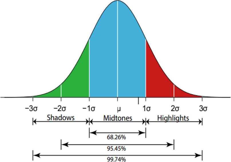
Pixel color distribution has been known to follow a normal distribution in a static scene that evolves over time [16, 22]. Consider an image pixel p acquired by a camera and located at coordinates (x, y) on the screen. During a fixed time period of n frames acquired, pixel p will show variations due to illumination effects. Our model defines four specific illumination ranges where pixel p moves across time.
The first range is referred to as the midtones range.
The mean intensity value of pixel p will be located in this range most of the time. The range below the mean value is named the shadows range. The following intensity range in the distribution is defined as the highlights range, and contains intensity values above the intensity mean of pixel p. A final range is defined outside of the three main possible ranges. This is the foreground range, where pixel intensity values differ drastically from previous gathered data.
Figure 1 shows the pixel normal distribution and the three proposed area ranges. Everything falling outside the [-3σ, 3 σ], interval will be labeled as a foreground object, not belonging to the original scene.
3.3 Sample Distribution with Unknown Population Parameters
For this particular application, both population mean and standard deviation are unknown quantities. Nevertheless, the algorithm must estimate a normal population with unknown mean µ and unknown standard deviation σ using the sample mean
A typical procedure is to replace σ with the sample standard deviation S [21]. However, the sampling distribution of the sample mean will no longer be normally distributed. Instead of using the random variable Z, that is, the standard normal distribution, it is possible to use a distribution called the t-distribution. The effect of replacing σ by S on the distribution of the random variable T is negligible if the sample size n is large enough. Commonly, a sample size between 30 and 40 is considered large enough [23]. The larger the sample size, the closer the t-distribution is to the z distribution. The shape of the t-distribution is very similar to the z-distribution: the contour is bell-shaped, the mean is zero, but the spread is larger.
3.4 Sample Size
Sampling is carried out during the training phase. During this stage the classifier gathers a pixel sample of a defined size n for parameter estimation. The condition of n > 30 is a common guideline if population distribution is not too far from normal [24]. As mentioned before, having an unknown population variance σ2 forces the algorithm to model the sample distribution as t-shaped. Nevertheless, the t-distribution resembles a normal distribution as sample size increases.
The choice of a meaningful sample size not only impacts on the classification results, but also consumes a fair amount of memory. During the training period, a number of frames equal to the sample size will be stored in system memory. Consider Table 1, where possible values of n are examined. It is possible to simplify some calculations if a sample size is chosen as a power of two (e.g., Sample mean µ computation involves a division by n). We have set the training sample size n to 32 (25) frames.
3.5 Pixel Population Mean and Standard Deviation Estimation
After defining a sample size with unknown parameters, population computation can be now formulated. Population expected value µ is estimated using an interval of plausible values.
The estimator comes in the form of a Confidence Interval (CI). This parameter is constructed so it offers high confidence that µ lies directly within this numeric range. The mean interval is built using a confidence level (1 − α) of 95 %.
The formal definition of a two-sided confidence interval on µ is:
where
Finally, it is possible to estimate the parameter σ by relying on the sample data obtained previously. The standard deviation of the population will be estimated by multiplying the square root of the size of the sample n by the standard deviation of the sample.
3.6 Population Distribution Segmentation and Classification
Once each pixel distribution has been estimated, the background model should offer reference information of both the population mean µ and standard deviation σ. This information is stored in a pair of matrices, indexed as the incoming pixels require. The next step in the process is to divide up the whole population distribution in the delimited regions used for pixel identification.
During classification, each pixel is evaluated according to its historical statistics. Each pixel is fitted in four possible classes: Shadows, Midtones, Highlights and Foreground. Figure 2 depicts the segmented pixel distribution.

We define six values used as thresholds for pixel comparison. Note that some threshold values in fact overlap, thus, it is possible to compute only four values instead of six. Each new pixel is labeled according to the following classification rule:
Additionally, each distribution threshold is computed using the µ CI previously built.
The lower mean value (µLower), can be used for lower thresholds and the upper mean value (µUpper) for upper thresholds. Both values can be either positive or negative. Each threshold value is computed as follows:
The prior operations are carried out during the classifier’s training phase. Resulting data such as pixel standard deviation mean and threshold information for each image pixel is stored in RAM memory. The classification phase is straightforward, as the background model is queried by each new pixel as the classification rule is applied over the whole image.
4 Results
The algorithm is first written and debugged as an embedded Matlab algorithm. Embedded Matlab is a subset of the Matlab computing language that generates C code directly from Matlab scripts. It can also be used to generate a Hardware Description Language (HDL), template through Simulink. Further C target-platform optimizations are carried out manually. Matlab offers us great developing tools and a complete insight of background classifier’s complexity running on an embedded environment.
We compare results obtained against two other methods often used as reference throughout literature: the Gaussian Mixture Model and the Horprasert algorithm. The latter has been developed by [25] and is used to benchmark of our own model. The entire database of test sequences includes seven video clips of small indoor and outdoor areas focused on low-traffic and varying environmental conditions (e.g., light, surfaces and objects). We have tested out-door and in-door scenes, where backgrounds can be either dynamic (i.e., moving objects such as trees are present) or static. Variable light is observed throughout all the videos, while traffic is labeled as low (1-3 persons) or medium (3-5 persons). Some scenes also feature reflective surfaces.
Figure 3 shows the first four scenes under testing, while Figure 4 depicts the last three scenes evaluated. The database used in the first five scenes is available online [26]. The sixth scene has been taken from the PETS2001 database [27] and presents an out-door surveillance view of a parking lot where no clean background of the scene is available, thus, the system is trained with cars already parked.

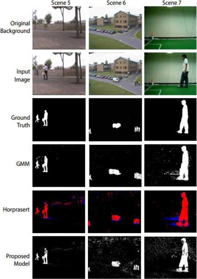
The Gaussian Mixture Model is tested using the following parameters: α = 0.005, ρ = 0.05 and three Gaussian distributions. The model does not include a shadow removal stage. MoG-classified pixels are colored white for foreground and black for background. The Horprasert decision parameters τCD, ταlo, τα1 and τα2 are selected threshold values used to determine similarities in chromaticity and brightness between the background model and the current image [18].
Parameter selection can be automatic or manual. In this application, the thresholds that achieved a better segmentation have been manually obtained through experimentation. The parameters used are: τCD = 5000, ταlo = −20, τα1 = 6 and τα2 = −6. Horprasert’s model classes are rendered in three colors: red for foreground objects, blue for shadows and black for background pixels. Our method’s results are shown using four different colors: white for foreground, gray for shadows, light gray for highlights and black for background pixels. All results are presented without any post-processing. Figure 3 and Figure 4 depicts the complete qualitative results of the input test database.
For quantitative evaluation, all seven video clips results are compared using the Percentage of Correct Classification (PCC), defined as follows:
In Equation (11), TP (true positives), represents the number of correctly classified foreground pixels; TN (true negatives) represents the number of correctly classified background pixels and finally, TPF represents the total number of pixels in a QVGA image.
The Ground Truth image is used as reference for measuring both the TP and TN values.
Table 2 depicts all the PCC values obtained for the seven tested scenes under the three different discussed methods. The maximum value of PCC is 100%, which indicates a result identical to the ground truth reference image. A lower result indicates a deviation from the ground truth.
Table 2 Quantitative comparison of PCC in % for each Background (BG) scene
| Method | BG 1 | BG 2 | BG3 | BG4 | BG5 | BG6 | BG7 |
|---|---|---|---|---|---|---|---|
| MoG | 91.14 | 98.67 | 99.45 | 98.68 | 99.36 | 97.37 | 96.82 |
| Horprasert | 97.61 | 98.84 | 99.47 | 99.35 | 98.23 | 98.32 | 97.53 |
| Proposed | 98.51 | 99.17 | 99.71 | 99.56 | 99.23 | 99.17 | 98.23 |
All methods are compared based on foreground and background classification; this means that shadows (or highlights) identified by the Horprasert model and our approach are rendered as background pixels for evaluation.
All methods are implemented on a PC with an Intel Core i3-2350M CPU running at 2.30 GHz with 4 GB of RAM running at a minimum of 30 frames per second. Estimated profiling using Matlab tools show a processing rate of 30 frames per second (average) with a system memory consumption of maximum 2.07 Mbits for background model storing.
Input is received as a sequence of 62 images compromising the video clips used in scenes 1, 6 and 7. The script has been separated in three main blocks: training, background model building and classification. The training block computes and stores the cumulative sum, minimum and maximum values of an incoming grayscale pixel for 32 frames. The background model building block computes the standard deviation and mean of all processed pixels. Finally, the classification block receives a grayscale pixel and outputs its classification label during 30 frames.
The final output of the full automatic surveillance system is shown in Figure 5. The system receives an input frame from the fixed-position camera. The background model constructs the Foreground Mask, where objects that do not belong to the original background are rendered in white. Shadows have been filtered out by the pixel classifier; this mask is then processed by a blob detection stage. Tracked blobs of interested are finally framed with a rectangle.

4.1 Discussion of the Results
Although our approach is developed mainly for in-door surveillance, we also tested performance under out-door conditions with reasonable reability. In the first scene we can observe the presence of dynamic multi-textured pixels (i.e., moving trees) among other environmental noises that hinder optimal segmentation. MoG achieves the best segmentation in the fifth scene, classifying correctly the dynamic pixels around the trees while optimally preserving the shape of the detected foreground objects.
Scene two and four present the noisiest environments in the database. Both sequences feature reflective surfaces and irregular light distorted by moving objects.
The reflection of the target objects (the persons walking through the hall) is identified in all three methods as entirely new foreground objects. In the second scene, MoG manages to filter out most of the noise produced by the composite surfaces (such as the building reflective walls and the blue moving fabric), while the floor reflections are better segmented using both the Horprasert model and our model.
While evaluating the third scene, the three techniques achieve a good segmentation with low background noise and good shape preservation. Enough shadow information is filtered out by Horprasert’s model and our approach, with no significant differences in both results. The sixth scene produces a lot of highlight and shadow noise with Horprasert’s model and our method. As mentioned before, this sequence has heavy light variations throughout the span of the video clip.
The seventh and final scene presents an interesting scenario, with uneven light and numerous shadows sources. MoG presents a lot of environmental noise; meanwhile most of the shadows are correctly identified by the Horprasert model. Our model also accurately identifies shadows and highlights present in the frame.
5 Conclusions
Background modeling is a typical computer vision task; however, algorithm implementations aimed for real-time embedded applications are limited. In this paper we proposed a background modeling algorithm with emphasis on real-time processing and memory savings. The background modeling algorithm relies on statistical information and is aimed for a fast implementation. It is developed as a supervised pixel classifier, where a background reference model is built during a training stage using a video sequence of a fixed background acquired by a stationary camera. Once trained, the system can actively classify the pixels of an input image in four different classes: background, shadows, highlights and foreground.
We compared the results obtained with two techniques that are often implemented on embedded platforms: the Gaussian Mixture Model and the Horprasert model. According to the tests conducted, the overall performance of our method is in-line with results obtained directly from software implementations. The impact of fixed-point operations in the proposed architecture is practically negligible while comparing with traditional statistical-based techniques.
Best classification results are obtained when the system monitors in-door areas with non-reflective surfaces, as reflective surfaces will introduce noise that can lead to miss-classified pixels. Under these circumstances noise can be minimized with the implementation of post-processing filters such as Gaussian, median, erosion and dilation. System accuracy can be generally boosted up by decimating the input stream of images. This will cause each N(µ, σ) tuple value to be extended to accept broader intensity values, reducing the possible noise obtained during certain scenarios.

