


 text new page (beta)
 English (pdf)
 Article in xml format
 Article references
 Send this article by e-mail
 Cited by SciELO
  Similars in
SciELO
Similars in
SciELO 
 Permalink
1 Introduction
Word sense disambiguation is usually defined as a task of detecting an exact sense in which a word is used from a set of possible word senses in a given context. In this paper the context is a dictionary definition of a noun sense, the ambiguous word within the definition is a hypernym of the defined noun sense and a set of possible senses is a set of dictionary definitions of the hypernym.
This kind of word sense disambiguation task arises in the process of lexical taxonomy construction. Here by lexical taxonomy we understand a directed graph where nodes represent word senses and edges represent hyponymy-hypernymy relations. Taxonomy forms core of many semantic resources: lexical databases, thesauri, ontologies. Such resources are widely used: they are vital as collections of word sense representations as well as part of many NLP tasks such as building a database of semantic similarity or as a tool for term generalization.
There are several kinds of approaches to create or update a taxonomy. A taxonomy can be manually created by lexicographers [16], converted from existing structured resource [20], extracted from a corpus [11] or derived from a corpus-trained vector semantic model [8]. Corpus extraction efficiency and methods vary greatly depending on corpus type with notable works done on corpora of dictionary glosses [21], formal text corpora [11] and large general corpora [19]. Each of the approaches is a trade-off between required labor and quality of the resulting taxonomy.
As a resource for taxonomy extraction a monolingual dictionary is a small corpus in a restricted language where most sentences contain a hypernym. Furthermore, the hypernym in most of these sentences occupies the same syntactic position. It is possible to create high-quality taxonomies by extracting hypernymy relations from such corpora [10]. The WSD problem described in this paper arose in the process of extracting a taxonomy for Russian language from a monolingual dictionary.
It is unclear whether WSD methods employed for the general corpora are suitable for this kind of WSD tasks. Thus in this paper we describe the results of applying several existing WSD method to the task of hypernym disambiguation in a monolingual dictionary definition. We test a range of possible configurations for each of the methods. The aim of the paper is to describe the parameters of the WSD methods that are the most important for solving the given WSD problem.
The rest of the paper is organized in the following way: it presents a brief overview of the existing approaches to the problem of WSD (section 2), then a description of the data sources, data preparation and annotation (section 3), a description of the WSD pipeline that compares different feature extraction and machine learning configurations (section 4), a description and an analysis of the most important WSD parameters and their performance (section 5), a discussion of the results (section 6) and finally a concluding summary of the presented work (section 7).
2 Background
Various approaches have been proposed to WSD task. All these approaches are based on the idea that it is context that defines the word sense, although the definition of what the context is varies.
One of the first WSD algorithms was proposed by Lesk [15]. Lesk introduced a metric of similarity between two contexts: the number of words present in both contexts. The algorithm performed well, but suffered from data sparseness: often the important context words are related but are not the same. The simplest solution to overcome this limitation is to use a semantic relatedness database. Thus Banerjee et al. [2] demonstrated a significant improvement over Lesk’s algorithm by using WordNet synsets to add more overlapping context words. Sidorov et al. [23] increase the number of matches between two context using an extended synonym dictionary and a dedicated derivational morphology system. This approach is reported to give high WSD precision on a corpus of Spanish explanatory dictionary.
Many attempts were made to incorporate machine learning in a WSD task, e.g. latent Dirichlet allocation [4], maximum entropy classifier [24], genetic algorithms [9] and others.
Approaches to WSD based on neural networks with autoencoder or similar topology date back as far as 1990 [25], however early approaches were impractical due to unacceptably high computational demands and slow and noisy learning algorithms. In 2013 Mikolov et al. [18] trained a large autoencoder — Word2Vec — and demonstrated similarity between arithmetic operations on autoencoder-derived word embeddings and some semantic relations. They also demonstrated superiority of Skip-gram model over continuous bag of words.
Word embedding model does not provide a single way to convert a word context to a feature vector. Iacobacci et al. [13] compared different approaches to extract word embedding features from corpus for WSD task. They tested several representations of a word sense: as concatenation or different weighted averages of word context vectors.
Many attempts were made to build a model of embedding word senses to a vector space, instead of words or lemmas. Iacobacci et al. [12] trained a Skip-gram model on a semantically disambiguated corpus, and Espinosa-Anke et al. [6] demonstrated usefulness of resulting set of vectors as a semantical relatedness database in a WSD task. Chen et al. [5] demonstrated that by iteratively performing WSD on a corpus using Skip-gram model and training the model on a resultant corpus it is possible to improve WSD performance over naive Skip-gram models. The suggested approach is very demanding in both time and memory required.
One of the first practical implementations of direct induction of word sense embeddings was put forward by Bartunov et al. [3]. The group created AdaGram, a nonparametric extension to Skip-gram model that performs bayesian induction of quantity of word senses and optimization of word sense embedding representations and word sense probabilities in the given set of contexts.
Recently recurrent neural networks entered the scene of NLP. Yuan et al. [26] put forward an approach to WSD based on LSTM neural network which presents a coarse model of how human beings read sentences sequentially. The network is trained to predict a masked word after reading a sentence. The word sense embedding vector to be used in WSD task is obtained from the internal representation of the word in the network.
In order to limit the scope of the work we restricted ourselves to just three models: Lesk model as a baseline, Skip-gram in Word2Vec implementation as a state of the art WSD model and AdaGram as a state of the art word sense induction model.
3 Materials
This work uses several sources of linguistic data available for disambiguation process: monolingual dictionary, ambiguous hyponym-hypernym pairs, vector semantic models. Part of ambiguous data was annotated to create a test dataset. These data collections are described below.
3.1 The Dictionary
Core source of lexical information is monolingual Big Explanatory Dictionary of Russian language (BTS) [14]. The dictionary contains 72,933 lexical entries and gives definition to 121,809 word senses, definitions are also given to approximately 24,000 phraseologisms. Of all information in the dictionary we only retain a set of noun word senses: 33,683 nouns with 58,621 senses overall. Word sense is represented as a lemma, word sense number, definition gloss, and extended gloss. The term “extended gloss” (or “gloss ext” in images) denotes definition with word usage notes and corpus examples.
3.2 Hyponym-Hypernym Pairs
Input to the WSD task is a list of pairs: hyponym-sense and hypernym-word. Hyponym is represented as a word sense, hypernym is represented as a word and a list of its senses. The tuples were extracted automatically from corpus of BTS word senses which is described in our previous work. Hypernymy is defined loosely in the dataset: the best hypernym-word was automatically selected from words present in definition gloss if any were available, but the algorithm did not check if there exist other words in the dictionary that are better hypernyms. The dataset is not organized as synsets. There are senses that a human expert considers synonymous, but in this work we ignore this fact and treat each word sense as distinct from all senses of other words. We also assume that all senses of any one word are different.
The dataset contains 53,482 hyponym-hypernym pairs. Hypernym is represented as a word, which may have 0, 1 or multiple senses defined in the dictionary. Hypernyms are more homonymous than random words: in the dictionary corpus for hypernyms an average number of senses is 3.0, for all nouns the average is 1.78 senses. If a hypernym has 0 or 1 senses, the task of disambiguation is trivial, such tasks are out of the scope of this paper. There are 39,422 hyponym-hypernym pairs such that a hypernym has at least two senses. In some cases one hyponym sense participates in pairs with several different hypernym words. Of such pairs only one is supposed to define true hypernymy relation. In the dataset there are 6,677 such hyponym-senses.
3.3 Data Annotation
In order to compare different WSD setups we need a reliable dataset (golden standard). To create such a reliable dataset disambiguation tasks were presented to two human annotators with linguistic background. To aid an annotator a dedicated annotation tool was created. The tool presents disambiguation tasks to annotators in a manner similar to the way the tasks are presented to WSD programs.
An annotator is presented with a hyponym word and gloss and a list of pairs of hypernym words and glosses. Hypernym might be expressed as different lemmas if such is given in the dataset or if the hypernym word has different possible lemmas. The annotator’s task is to select the gloss that most precisely expresses the hypernymy relation. For each hypernym candidate the annotator assigns a score of 5 to the exact hypernym, 4 to an indirect hypernym or a sense that is difficult to distinguish from the direct hypernym, 3 to a far indirect hypernym, 0 to the other senses. The annotator also has several options to reject the WSD task altogether: if due to POS-tagger error hyponym is not noun, if there is no suitable hypernym word, if there is no gloss suitable for hypernym sense.
The annotation tool is designed to annotate as long hypernym chains as is possible starting from a given pool of hyponyms.
For this purpose after any answer the tool selects one of hypernyms with the score of 5 and presents it to the annotator, if any such answer exists and was not annotated by the same person previously. If no such hypernym is found, the next question presented to the annotator is selected from the pool.
In the case where annotators doubt whether a given sense is a hypernym sense or a synonym sense, they are permitted to assign a good hypernym score to the sense. This may lead to a cycle in the chain of hypernyms. If such cycle occurs, then every sense in the cycle is either hypernym or synonym to every other sense in the cycle. This is only possible if all senses in the cycle are synonymous. So by allowing the annotators to be less strict in distinguishing hypernyms and synonyms we get a simple way to detect some synsets.
Disambiguation task is formulated as a multiple-choice question. This makes it difficult to assign correct answers based on majority votes of annotators. Instead, we retain answers of both annotators and marks assigned to specific hypernym senses. Thus we are able to create a strict and a lenient dataset by selecting either minimal or maximal score and retaining only hyponyms for which at least one hypernym has positive score. Raw dataset contains 1,537 hyponym-hypernym pairs annotated by at least one person, of those 646 were annotated by two persons. Some of the tasks are rejected by annotators: of 646 tasks annotated by two persons only 342 were not rejected by at least one annotator. The small intersection of annotated pairs is in part due to the annotation procedure described above: if annotators initially choose different hypernyms, then they annotate different hypernym chains.
WSD is a difficult task yielding low, but positive annotator agreement. We employed two metrics for inter-annotator agreement. For lenient agreement percentage we counted the fraction of WSD tasks for which there exists at least one sense that both annotators marked as acceptable (score greater than 0). Strict agreement is the fraction of WSD tasks for which the highest-scoring senses are the same.
For the given annotation task lenient agreement is 52%, strict agreement is 19%. For a more descriptive agreement metric we calculated Fliess κ metric [7]. To do this we translated annotator reply for each answer to 0/1 score. For lenient metric 1 corresponds to any positive score, yielding κ = 0.34±0.06. For strict metric 1 corresponds only to answer 5 for both annotators, yielding the same value κ = 0.34 ± 0.06.
3.4 Embedding Models
In this paper, we compare the performance of two embedding models: a word embedding Word2Vec Skip-gram model and a word sense embedding AdaGram model. Both models are trained on a 2 billion token corpus combined from RuWac, lib.ru and Russian Wikipedia [17]. The corpus is tokenized and lemmatized with mystem3 [22], lo-wercased and cleared of punctuation. Parameters for Word2Vec are: 300-dimensional embeddings based on 5 word context, the dictionary includes words of frequency 10 and above. AdaGram model stores vector embeddings for every word sense resulting in several-fold larger memory requirements.
To compensate for large memory footprint we restricted included word frequency. Parameters for AdaGram are: 300-dimensional embeddings based on 5 word context, dictionary includes words of frequency 100 and above. To estimate whether such restriction is hindering the model performance we annotated a corpus of 100 random words that have training corpus frequency between 10 and 100. Of 100 words 32 were identified as actual words, of those 3 were vernacular, 12 - numerals or dates, 17 - rare proper names, other words include 7 errors of lemmatization, 5 words from different language or obsolete words, 36 words were incomprehensible to the annotator.
After accounting for frequency we expect the model to omit no more than 0.000,8 of context words on dictionary corpus and consequently to exhibit virtually it’s best performance.
4 WSD Experiment Setup
The overall structure of WSD pipeline is the following: (i) parse and group the data to form WSD batch tasks, (ii) for each batch represent each word sense in the batch as a feature vector, (iii) apply machine learning to predict hypernym sense for each hyponym sense in the batch, (iv) choose one hypernym lemma if several alternative hypernym lemmas are given. For steps (ii) and (iii) different implementations were tested. Some of the step implementations have configurable variables. The goal of the experiment is to perform a grid search over all reasonable configuration variable combinations.
Human annotators displayed better performance when given a batch of WSD tasks with the same hypernym. Our intuition is that human annotators notice similarities in hyponyms and this gives them ability to apply the same answer to the whole group of similar hyponyms. In this work we attempt to simulate this behavior in automatic disambiguators. To achieve this the step (i) of WSD is to collect a batch of all senses of some lemma (hypernym) and all senses that are hyponyms to the given lemma. The WSD task is then formulated in the following way: every hyponym and hypernym sense in the batch is transformed to vector representation and every hypernym sense is annotated with “correct answer”: it’s sense number.
The goal of WSD is to annotate hyponyms with sense numbers. This is very similar to supervised machine learning with only one training point per class. It is important to note that the task is not actually supervised: the formulation provides no ability to somehow inject known correct hyponym-hypernym pairs to allow the disambiguators to adjust their answers. Within this procedure semi-supervised algorithms attempt to cluster hyponyms before annotating each cluster with hypernym sense — a behavior similar to assumed human annotator behavior. As described below, here we test both supervised and semi-supervised machine learning methods to achieve the best possible performance when comparing selected features.
The goal of step (ii) (feature extraction) is to assign a feature vector to each word sense using it’s definition gloss. This process varies depending on the embedding model selected: either Lesk, Word2Vec or AdaGram:
— Lesk model assigns an embedding vector to a word use context. Head word sense embedding represents number of occurrences of each word in the sense definition gloss. For the model we vary which parts of the definition are used: any of head word, gloss, extended gloss.
— Word2Vec model assigns a vector to a dictionary word. Given such model we search for a word sense definition vector in form of a weighted sum of selected words from the definition. We vary which parts of the definition are selected (any of headword, gloss, extended gloss) and weighting schemes: equal weights, TF·IDF weights and equal weights in a ±5 window around hypernym mentions.
— AdaGram model defines pre-trained word sense embeddings and derives word sense probabilities from word context. To obtain a head word sense embedding we put it in the context of its definition. In this case we define two variables: what part of the definition to use as a context (gloss or extended gloss) and how to account for the predicted word sense probability distribution (to use most probable embedding, to use weighted sum of embeddings according to sense probability, or to use sense probabilities vector as a nonsense embedding vector).
A batch of vector representations of word senses is then sent to a classifier with a task to annotate each hyponym with hypernym sense number, step (iii).
We test three classifiers: the nearest vector prediction, and two semi-supervised classifiers: label spreading and label propagation [27]. For each learning method a logarithmic grid search of reasonable variable values was performed. Be-sides method-specific variables described above, the only variable on step (iii) is kernel, with values: euclidean, cosine and RBF. For RBF kernel a range of values for γ was evaluated.
For each variable described in this section we followed the rule: if the best-performing value is extreme in it’s range then the range of values tested is extended. Adding a few values to several value ranges results in considerable increase of the overall grid search time. To avoid this in many cases the grid search step was increased instead of increasing the number of tested values in the range.
5 Results
In this section we define the scoring approach, then present the best performing algorithm, and then describe influence of selected features on the WSD accuracy.
For scoring we employed the lenient dataset described in section 3.3: score for a reply option is a maximum of scores given by annotators to this option.
Annotators’ scores are translated to the interval [0, 1] to give 1 to the best answer and exponentially lower scores to imperfect correct answers: s=2h−132 where h is a human annotator reply in the range [0, 5], s is the accuracy score used in calculations below. Algorithm accuracy is the average score assigned to its answers.
The best performing algorithm achieved an average accuracy score of 0.6. The best accuracy is achieved by label propagation predictor with RBF kernel using skip-gram word embeddings weighted according to the word TF·IDF value, word sense context obtained from the weighted sum of the gloss with the extended gloss and more weight given to the gloss.
Table 1 shows the best scores of different disambiguator configurations that employ a given combination of the selected language model and parts of definition that were used for feature extraction. Many tested distributive semantic model configurations outperform the classic Lesk features. We may infer that distributive models are suitable for the task given: WSD of hyponym-hypernym relations based on a corpus of dictionary definitions. Within the scope of this work only the classic version of Lesk features was tested as the baseline. Based on the published data [1] we expect the distributive semantic models to outperform the better of modifications of Lesk features too.
Table 1 Importance of language models and feature sources for WSD accuracy
| part | gloss | gloss_ext | ||||
|---|---|---|---|---|---|---|
| max | mean | std | max | mean | std | |
| model | ||||||
| AdaGram | 42% | 33% | 5% | 40% | 31% | 5% |
| Lesk | 32% | 25% | 7% | 45% | 29% | 9% |
| Word2Vec | 50% | 37% | 4% | 59% | 41% | 8% |
Surprisingly, the AdaGram model that won one of RuSSE tracks was outperformed by both Word2Vec and baseline Lesk models, so these results require further investigation. It might indicate that the model requires some fine-tuning for use in dictionary-based WSD. Otherwise, this might mean that different approaches to incorporate word sense embeddings into machine learning features are needed.
Dictionary includes different types of information that can serve as a context for the disambiguation task: head word, gloss, usage notes, corpus examples. Of that information we further use a head word, a gloss and an extended gloss (which is gloss with usage notes and corpus examples). Table 2 shows the accuracy of disambiguators depending on what kind of information they were presented. Notably, accuracy is improved by using as much context as possible. This stands in contrast with a general corpus-based WSD where some context restriction is required to obtain the best performance [13].
Table 2 Importance of different dictionary entry parts for WSD accuracy
| max | mean | std | |
|---|---|---|---|
| part | |||
| gloss | 46% | 37% | 4% |
| gloss and head | 50% | 38% | 5% |
| gloss ext | 59% | 40% | 8% |
| gloss ext and head | 59% | 42% | 8% |
| weighted gloss and gloss ext | 62% | 42% | 9% |
One can assume that the main reason for good accuracy of extended glosses is that they include corpus examples, which give better contexts for the hypernym.
We argue that not only corpus examples contain valuable information, but the gloss itself is also important. To verify this we extracted a weighted average of gloss embeddings and extended gloss embeddings. For this test we only use Word2Vec as the best performing model. Weighting is done as vw (G, Ge) = w · v(G) + (1 − w) · v(Ge) where w is the weight, G is a gloss, Ge is an extended gloss, v(G) is the embedding of a gloss, and vw is the weighted average. Figure 2 demonstrates how WSD accuracy depends upon weight value. Here the best accuracy is achieved at weight of approximately 0.5.

Fig. 1 Distribution of accuracy exhibited by different disambiguator setups grouped by features used for disambiguation
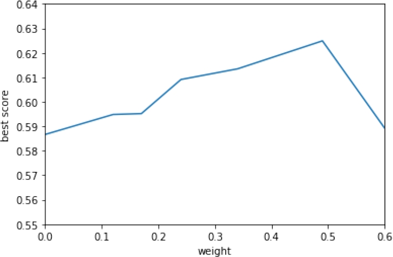
Fig. 2 Best accuracy of WSD algorithm depending on weighting gloss and extended gloss. Features used for classifications obtained as vw(G, Ge) = w · v(G) + (1 − w) · v(Ge) where w is the weight plotted, G, Ge are gloss and extended gloss, v, vw are embedding functions
Figure 1 shows the accuracy of different feature selection approaches as violin plots. Here Y axis always displays the score of the corresponding approach and the width of a violin shows the number of algorithms employing the approach that performed up to the given score. The widest part of a violin is the expected accuracy of a random WSD algorithm that just uses the given approach and random values for all other configurations: the lower this value is the more fine-tuning the algorithm demands. If there is a widening at the top of a violin, then the selected approach is one of the most important properties of the disambiguator and there are some irrelevant variables in the algorithm configuration. If the top of the violin is narrow, then the best performance is either a chance event or relies upon very delicate configuration tuning.
6 Discussion
Figure 3 demonstrates examples of hypernym chains obtained with one of the best performing algorithms. Without thorough scrutiny we may note that the fraction of incorrect hypernym chains is intolerably large. Here by incorrect hypernym chain we understand a hypernym chain that contains at least one error. Such hypernym chains are not suitable for fully automatic taxonomy generation. Errors are not grouped in one part of the lexicon and are spread all over the dataset. Figure 4 shows examples of senses identified as co-hyponyms.

Fig. 3 Examples of hyponymy chains. Left column contains transliterated Russian examples, right column provides English translations. With WSD accuracy near 0.6 and errors spread uniformly around the corpus 95% of the resulting hyponymy chains longer than 6 hyponyms have at least one error

Fig. 4 Examples of co-hyponym groups for different senses of lemma ST’EP’EN’ (DEGREE). In each table the top row is a hypernym sense, the rest are examples of hyponym senses selected by the WSD for the hypernym sense. Left column contains transliterated Russian examples, right column provides English translations. The examples illustrate that co-hyponyms are typically grouped together correctly
Here we see that many large sets of co-hyponyms are correctly grouped together, even though sometimes they are attributed to a wrong hypernym sense. This calls for a metric that gives a number of edit operations necessary to obtain the correct taxonomy graph. The metric might favor different WSD approaches than those reported in this paper. One can expect that such metric will further prefer methods based on clustering or semi-supervised learning to other methods.
Of the 808 WSD tasks that have at least one answer accepted by annotators, 768 were correctly solved by at least one disambiguator configuration. This allows us to speculate that even without any improvement of the selected features it is possible to greatly increase accuracy by using ensemble methods. This way the accuracy values within range between the achieved 0.61 and the theoretical limit 0.97 might be reached.
7 Conclusions
The task of a hypernym WSD in a monolingual dictionary is an important task that is considerably different from a general corpora WSD. As in general corpora, some distributive semantic models show good accuracy in this context. Surprisingly, AdaGram, one of the best performing models for general corpora, did not perform better than the baseline Lesk algorithm. Reasons for such poor accuracy of AdaGram model require further investigation.
Monolingual dictionary definitions provide strong boundaries to word contexts. We show that in this case WSD benefits from using the whole available context, as opposed to a general corpus where narrowing the context is necessary to achieve the best performance. We also show that while corpus examples in monolingual dictionary are an excellent source of context information, definition glosses contain more valuable features. A more detailed comparison of WSD accuracy on general corpus, dictionary corpus examples and definition glosses might explain some differences in disambiguator’s behavior.

