


 text new page (beta)
 English (pdf)
 Article in xml format
 Article references
 Send this article by e-mail
 Cited by SciELO
  Similars in
SciELO
Similars in
SciELO 
 Permalink
1 Introduction
A bilevel optimization problem has two levels of single or multi-objective optimization problems such that the optimal solution of the lower level problem determines the feasible space of the upper level optimization problem. In general, the lower level problem is associated with a variable vector
However, the upper level problem usually involves all variables
From the economic viewpoint they can be seen as decision making scenarios where an upper-level leader is optimizing a strategic (main) model, while a lower-level follower reacts to the leader decisions by optimizing a related subproblem. In other words, they are “mathematical programs with optimization problems in the constraints” [7]. BOPs have been extensively studied in the past (e.g. location routing problems [19], relief operations after a disaster [5], Stackelberg games [27], engineering problems [14], among others). Even in more simple cases (e.g. models with linear objective functions and constraints) BOPs are hard to solve by traditional optimization techniques [11, 12].
Nowadays, the use of metaheuristic methods to deal with bilevel optimization problems is gaining increasing attention [30]. One of the reasons behind this interest is their ability to obtain near optimal solutions in a reasonable amount of time [3]. Moreover, as these methods are derivative-free, they could be applied to solve non-differentiable problems.
As in other optimization scenarios, uncertainty may exist, being one source of it, the dynamic nature of data involved in the mathematical model. Examples of these dynamic BOPs (DBOPs), could be location routing problems with variable number of depots or clients over time, or aid distribution in recurrent disasters, among others. This feature increases the complexity of BOPs, since now the goal of any solving strategy is to find the optimal bi-level solution (or the best possible achievable solution with the available resources), at every time step. Despite the importance of studying these special scenarios, the literature reflects just a few works addressing this topic.
For example, in [29] a genetic algorithm is used to solve a dynamic traffic signal problem. The authors were focused on modeling the decision scenario of dynamic traffic signal optimization in networks with time-dependent demand and stochastic route choice. Here, the upper-level problem represented the decision-making behavior (signal control), of the system manager, while the user travel behavior is represented at the lower level.
[18] proposed a general model for dynamic bi-level multi-objective problems. The authors analyzed the interaction between the upper and lower levels over time and described the benefits of bi-level dynamic multiobjective optimization through the examination of an industrial case in which the design of a paper mill (upper level) and the mill operation (lower level), are optimized. As solution method, the authors considered a differential evolution algorithm.
Another study on dynamic bi-level optimization was conducted by [6]. Authors addressed the modelization and solution of a multi-period portfolio selection problem in stochastic markets with bankruptcy risk control. They assumed that the investor wants to find an investment strategy to maximize his terminal wealth, while the bankruptcy risk in each period needs to be controlled. Essentially, a bi-level programming algorithm is employed for deriving analytical solutions for the each period-wise optimization problem.
In this context, we propose to deal with these complex scenarios by exploiting the current advances on metaheuristics methods from the fields of bi-level [30] and evolutionary dynamic optimization [1]. To the best of our knowledge, there are no research works related to this topic.
More specifically, in this paper we address the solution of dynamic bi-level optimization problems by hybrid metaheuristics. Our hypothesis is that, by hybridizing successful solving approaches from both bi-level and dynamic optimization fields, an effective method for solving DBOPs can be obtained. We will focus on coevolutionary and multipopulation methods, which are successful strategies for tackling bi-level and dynamic problems, respectively [30, 16].
The rest of the paper is organized as follows: Section 2, gives the necessary background on DBOPs. Section 3 describes the proposed method for solving DOPs, which is validated through computational experiments in Section 4. Finally, some concluding remarks and future works are outlined in Section 5.
2 Background and Related Works
This section is devoted to the fundamentals of dynamic bi-level optimization problems. In order to better understand the formulation of DBOPs, we start by defining bi-level and dynamic optimization problems. Furthermore, we summarize some available metaheuristic based solution approaches. The section ends with the definition of the dynamic bi-level optimization problems.
2.1 Bi-level Optimization Problems
A bi-level optimization problem is defined as follows:
where
For example, for a given value of
We will now illustrate a real-life BOP model through an example. We consider the Stackelberg competition model described by [26] in the context of game theory.
Example 1 (Stackelberg competition) Two firms (
where
Solving this model implies for the leader firm
Now suppose that both firms sell homogeneous goods and their corresponding price functions
where
where
[26] shows that it is possible to analytically compute the optimal solution, which is given by:
We can interpret these values as the optimal strategies of the leader and follower at Stackelberg equilibrium.
From the viewpoint of metaheuristic met-hods, BOPs can be solved using the following approaches [30]: (1) nested sequential, (2) single-level transformation, (3) multi-objective, and (4) coevolutionary.
The first one is the most intuitive but the most computationally expensive, since for every single evaluation of the upper-level objective function, the lower-level problem needs to be solved. To cope with such complexity, other authors transform the bi-level problem into suitable models that can be solved by other metaheuristics (e.g. genetic algorithms, multi-objective evolutionary algorithms, etc.), which is the case in the second and third approaches.
However, note that these approaches can be applied under the following conditions: 1) an explicit model of the problem is known and 2) there exist some proof that such transformations lead to the true (or near), optimal solution of the problem.
Finally, the more general approach is to use coevolutionary algorithms (CoEAs). Here, the algorithm evolves two populations (sets) of solutions for both, the upper-level and the lower-level problems. In addition, CoEAs must implement some exchange mechanisms for guiding the search process. Defining such mechanisms is a key issue in the algorithm performance on BOPs. We will return to this topic in Sec. 3.
2.2 Dynamic Optimization Problems
A dynamic optimization problem (DOP), is formally defined as:
where
In this dynamic context, the main goal of a metaheuristic is to find the best solution at every time step. Between changes, the problem is “static” thus allowing the algorithm to perform the optimization process. So, keeping a suitable level of diversity in the population is a challenge when using population-based metaheuristics in dynamic environments. A proper management of diversity allows for avoiding premature convergence in previous environments and for tracking the new optima after the change.
Regarding of how this challenge has been addressed in the past, [13] and [8] observed four strategies: 1) enhancing diversity after the change, 2) maintaining diversity during run, 3) memory-based approaches and 4) multi-population approaches. More recently [21] pointed out that another alternative is to implement self-adaptive strategies [20] to cope with changes. This latter approach provides the algorithm, the ability to intelligently react to environment variations, as was shown by [22, 24].
2.3 Dynamic Bi-level Optimization Problems
From the previous definitions (1) and (9), it is straightforward to derive a general formulation for dynamic bi-level optimization problems:
Here, note that there are two sets of system control parameters,
BOPs where both subproblems are stationary,
DBOPs with dynamism only in the upper-level problem,
DBOPs with dynamism only in the lower-level problem and
DBOPs with dynamism at both levels.

Fig. 1 Possible bi-level optimization problems according the type (stationary or dynamic), of the lower-level and upper-level problems
The most difficult scenario arises when both subproblems are dynamic.
In order to illustrate a DBOP, we derive the dynamic version of the problem described in Example 1 from Sec. 2.1.
Example 2 (Dynamic Stackelberg competition)
From model (2), suppose that firm
where
where
One important question here is how the optimal solution of the model is affected when these system control parameters change over time. By using the general expressions (6 - 8), for the optimal solutions, we can have an idea of how it can be affected. In that sense, Figure 2, shows what happens in a hypothetical scenario, in which the model changes 10 times and the other parameters takes fixed values as follows:
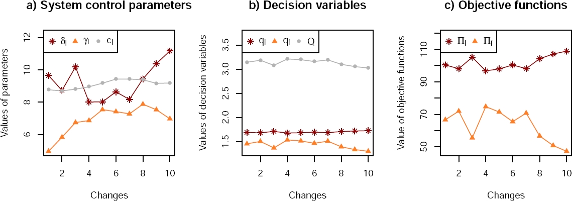
Fig. 2 Effects of changing system control parameters over time a), on decision variables b) and objective functions c), for the optimal solution
Figure 2, shows the effect of varying
The reader must be aware that real-life DBOPs can be more complex than this illustrative model. For instance, models in higher dimension, with stronger interactions among decision variables [26], could not be solved by analytical or numeric techniques. Besides, if the change function (e.g. Eq. 12) and the frequency of such changes are not known, then we must to rely on approximation optimization methods for finding near optimal solution quickly, that is, before the occurrence of a new environment in the near future. In what follows we explain our proposal to deal with such scenarios.
3 Proposed Approach
As mentioned before, coevolutionary algorithms (CoEAs), are among the most general approaches for tackling BOPs. In this context, a successful experience has been recently reported by [15]. Basically, a CoEA performed a pairwise optimization process (coevolution), by exploiting the separable structure of the problem at hand. Usually this is the case in bi-level optimization problems.
On the other hand, in the context of dyn-amic environments, using multi-population and self-adaptive approaches have shown to be very effective [9, 22, 24], specially, when combined with the differential evolution metaheuristic [28]. While the use of several populations enables a proper exploration of the search space, self-adaptation contributes to enhance the algorithm diversity and the optimum tracking over time.
From these facts it is reasonable to expect that a suitable method for solving DBOPs should involve a combination of the above approaches. In this sense, we propose a hybrid metaheuristic that comprises a simple coevolutionary approach based on the works of [25, 15] and the mSQDE algorithm from [22]. Specifically, mSQDE is a self-adaptive, multipopulation algorithm proposed for dynamic optimization. We have based our selection on the reported success of such approaches in their respective domains.
Figure 3, outlines the general structure of the proposed method, named CoEvoMSQDE. Note that CoEvoMSQDE acts as a coordinator by deciding what, when and how the coevolution process is carried out. Two mSQDE algorithms/instances, denotes as

Each mSQDE is composed by a set of populations and every population comprises a set of solutions to the problem at hand.
As pointed out by [30], stating what, when and how is a key issue in designing CoEAs. So, here we explore different mechanisms. Specifically, regarding what information is exchanged, we consider three alternatives:
The global best solution of mSQDE instances (
The best solutions of sub-populations of mSQDE instances
All solutions of the best sub-population of mSQDE instances
Regarding how the exchange process is carried out, we consider the following alternatives:
Exchange with preference in the upper-level algorithm. We refer to this scheme as u. The upper-level algorithm is updated with the current best solution of the lower-level algorithm. Then, all solutions of the upper-level algorithm are evaluated and its global best solution is updated. Finally, this new global best solution of the upper-level algorithm is sent to the lower-level algorithm.
Exchange with preference in the lower-level algorithm. Referred as l. It operates as the previous scheme, but using the lower-level algorithm first.
Exchange without preference. Referred as w. The algorithms exchange their current best solutions, without intermediary evaluation and selection process.
With the aim of illustrating these alternatives, Fig. 4, shows them through task diagrams over time. Please note that the operation involved in these schemes are marked by different tonalities.

Finally, regarding when the exchange process will be done, we simply do it after a predefined number of iterations.
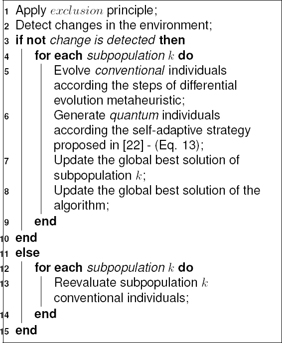
The main steps of the CoEvoMSQDE method are depicted in Algorithm 1. Note that the first two steps are devoted to set the problem definitions to the instances

Specifically, the iterative process of algorithms
Regarding to the self-adaptive strategy of mSQDE it is important to state that it has been defined as class of self-adaptation applied to the mechanisms for DOPs [24]. More specifically, it includes self-adaptation into the diversity during the run mechanism. Such mechanism is based on the generation of the so-called quantum individuals proposed by [2]. In the original scheme, these random individuals are generated in a hypersphere with a predefined radius
Formally, be conventional individuals denoted as
where
It can be observed that a new
The above features are depicted by Algorithm 2. For more details, the reader is referred to [22, 24].
4 Computational Experiments and Results
The main goals of the computational experiments are: to study the information exchange mechanism proposed and to analyze the performance of our coevolutionary approach for solving BDOPs.
In order to evaluate our approach, we need test problems that not only fit the model given in Eq. 10, but also involve the three scenarios identified in Sec. 2.3. To the best of our knowledge, such test problems are not available, thus we will use existing dynamic functions for the upper level and lower level subproblems.
In this sense, one suitable candidate is the well-known Moving Peaks Benchmark (MPB) [4], specially the so-called Scenario 2 which offers a multimodal objective function composed of several peaks.
In turn, every peak
where
In general,
Based on the model of DBOPs given in (10) and the MPB’s objective function of Eq. 14 we can derive the following scenarios:
Here, objective functions
4.1 Description of the Experiments
We divided the experiments in two groups according to our goals:
The effect of the exchange mechanisms in the three BDOPs scenarios and
The performance of the best variants of CoEvoMSQDE algorithm in more complex scenarios.
In the first group we tested the exchange mechanisms previously described, in the scenarios
Table 1 contains the parameters setting used for the subproblem instances
Table 1 Parameters setting for subproblem instances
| Parameter | Setting |
| Dimension |
5 |
| Search space |
|
| Number of peaks | 10 |
| Peak heights |
|
| Peak widths |
|
| Peak function |
|
| Shift severity |
1.0 |
| Change frequency |
5000 |
| Correlation coefficient |
1.0 |
Regarding the parameters setting of the CoE-voMSQDE algorithm, note that we have two levels. At the top level, we have the exchange mechanism (that we will study next), while at the bottom level, we have the mSQDE instances which will use the same parameter settings suggested by [22]. Specifically, the mSQDE instances will be composed of 10 sub-populations, each having 10 individuals (i.e. 5 conventional and 5 quantum ones). The scaling factor and the mutation probability affecting the self-adaptive strategy, were defined as
Defining a suitable performance measure for assessing the behavior of an algorithm, in both bi-level and dynamic optimization environments, is currently an active research area. In the case of bi-level optimization, [30] suggests employing error rates for the upper-level and lower-level objective functions in case the true optimums of both functions are known. When the optimum is not known, in [15] proposed rationality-based measures.
On the other hand, in dynamic environments several measures exist, the offline error [4] and the best error before the change [17], being two of the most employed. While the offline error indicates the average performance of the algorithm at every time step, the best error before the change only takes into account the last time step before a new change occurs in the environment. In any case, choosing the right measure primarily depends on the research goal. In our case, we are focused on assessing the algorithm performance in those time periods where the problem remains unchanged, so the best error before the change results appropriate. Formally, this measure is defined as:
where
We performed 30 runs for each pair of problem-algorithm instance, using different random seeds. Besides, we assumed that each problem instance would change 100 times every
4.2 Influence of the Exchange Mechanism
In this group of experiments, the goal is to analyze the influence of the exchange mechanisms consi-dered in the CoEvoMSQDE algorithm. Remember that the exchange mechanisms are composed of the when, the what and the how strategies.
Statistically speaking, such strategies will be the factors of the experiments and we consider three levels for these factors. In the case of the what and how the strategies described in Sec. 3 were selected, while for the case of when, the number of iterations between exchanges will be
These 27 variants were tested in scenarios
Figure 5 shows the average ranks obtained by the 27 variants that we considered. Note that we have divided the analysis in four main groups: results in scenario

Fig. 5 Effects of different coevolutionary schemes for each BDOP type, in terms of the average ranking of the variants according to the Friedman test
In these graphs we highlighted with a black bar those variants with the best average rank. For instance, in the scenario
Despite the relevance of these specific conclusions, the major observation here is the influence of what information is exchanged and when. For example, when the exchange is made every 1 iteration, the variants performance is low, regardless of the problem instance. This could be an obvious fact if we take into account that both,
On the contrary, variants with exchanges every 10 and 20 iterations are much better, since the populations have more time to evolve. To better understand this aspect, recall that the problem instances we considered change every 5000 function evaluations. On the other hand, our tested variants used 202 function evaluations at every iteration (since
Similarly, the type of information exchanged has a relevant impact on the algorithm’s performance. From the results obtained, it is worth noting that exchanging the global best solution

Fig. 6 Evolution of the best error before the change for variants of the form
The plots in left column (e.g. Fig. 6-a, c and e), correspond to the upper-level subproblem. On the other hand, the plots in the right column (e.g. Fig. 6-b, d and f), show the evolution of this measure for the lower-level subproblem, where the objective function is
Finally, in contrast with the when and what schemes analysis, results showed that no sub-stantial differences exist regarding how to perform the exchange. However, a slight advantage is observed for the
The experiments in the next section will focus on this aspect.
4.3 Results in More Complex Scenarios
Based on the previous results, we will explore the performance of successful variants of the proposed method over more complex scenarios. Specifically, we focus on the variants using:
In this experiments, we just focus on the
We consider the following peak functions:
In the former case, we consider different combinations of these functions (including
Next and using just the function
The possible dimensions are
The results in terms of the average best error before the change are shown in Tables 2 and 3.
Table 2 Mean of the best error before the changes ± standard error in the
| Upper-level |
Lower-level |
10+g+u | 10+g+l | 10+P+u | 10+P+l | 20+g+u | 20+g+l | 20+P+u | 20+P+l |
| Cone | Cone | 3.58±0.10 | 3.46±0.08 | 5.51±0.14 | 5.30±0.11 | 3.76±0.09 | 3.88±0.09 | 5.73±0.11 | 5.54±0.09 |
| Sphere | 2.71±0.09 | 2.63±0.09 | 4.69±0.13 | 4.42±0.11 | 3.00±0.07 | 3.08±0.08 | 5.07±0.08 | 4.76±0.10 | |
| Quadric | 3.51±0.11 | 3.45±0.10 | 5.55±0.16 | 5.29±0.12 | 3.83±0.08 | 3.77±0.07 | 6.00±0.13 | 5.64±0.12 | |
| Schwefel | 4.69±0.11 | 4.51±0.10 | 6.91±0.25 | 6.58±0.12 | 4.86±0.10 | 4.88±0.09 | 6.95±0.10 | 6.97±0.11 | |
| Sphere | Cone | 2.17±0.07 | 1.99±0.04 | 4.54±0.23 | 3.93±0.13 | 2.64±0.06 | 2.55±0.05 | 4.79±0.12 | 4.45±0.10 |
| Sphere | 1.47±0.06 | 1.24±0.05 | 3.65±0.27 | 2.99±0.08 | 1.91±0.06 | 1.79±0.06 | 3.85±0.18 | 3.77±0.11 | |
| Quadric | 2.35±0.07 | 2.16±0.07 | 4.77±0.27 | 4.10±0.14 | 3.45±0.19 | 3.32±0.18 | 5.95±0.28 | 5.87±0.26 | |
| Schwefel | 3.30±0.09 | 3.12±0.08 | 6.09±0.40 | 4.99±0.10 | 3.71±0.09 | 3.61±0.10 | 6.28±0.22 | 5.61±0.20 | |
| Quadric | Cone | 3.41±0.09 | 3.14±0.07 | 8.71±2.03 | 5.38±0.15 | 3.71±0.07 | 3.62±0.08 | 6.16±0.16 | 5.95±0.11 |
| Sphere | 2.65±0.09 | 2.42±0.07 | 7.42±0.97 | 4.59±0.11 | 3.01±0.08 | 2.90±0.08 | 5.90±0.38 | 5.20±0.08 | |
| Quadric | 3.48±0.09 | 3.30±0.08 | 7.64±0.96 | 5.75±0.12 | 4.69±0.18 | 4.61±0.19 | 7.61±0.35 | 7.16±0.22 | |
| Schwefel | 4.46±0.11 | 4.28±0.11 | 8.71±0.61 | 6.56±0.16 | 4.72±0.10 | 4.56±0.12 | 7.56±0.14 | 7.19±0.14 | |
| Schwefel | Cone | 4.87±0.15 | 4.51±0.11 | 8.52±0.72 | 6.92±0.13 | 5.40±0.14 | 5.43±0.14 | 7.86±0.13 | 7.78±0.13 |
| Sphere | 3.99±0.11 | 3.76±0.12 | 7.38±0.62 | 6.12±0.15 | 4.95±0.14 | 4.93±0.15 | 7.60±0.17 | 7.40±0.19 | |
| Quadric | 6.37±1.44 | 4.77±0.14 | 12.09±1.84 | 7.41±0.19 | 7.20±0.30 | 7.19±0.30 | 10.11±0.39 | 10.02±0.41 | |
| Schwefel | 5.81±0.16 | 5.49±0.13 | 8.73±0.34 | 8.03±0.21 | 6.36±0.14 | 6.33±0.13 | 9.08±0.19 | 8.97±0.13 |
Values in bold-face correspond to the best variant.
Table 3 Mean of the best error before the changes ± standard error in the
| Upper-level |
Lower-level |
10+g+u | 10+g+l | 10+P+u | 10+P+l | 20+g+u | 20+g+l | 20+P+u | 20+P+l |
| 2 | 2 | 1.16±0.07 | 0.62±0.03 | 2.49±0.09 | 1.85±0.06 | 1.00±0.04 | 0.85±0.03 | 2.23±0.04 | 2.12±0.06 |
| 5 | 1.82±0.06 | 1.43±0.03 | 3.28±0.06 | 2.74±0.04 | 1.81±0.04 | 1.55±0.03 | 3.30±0.06 | 3.13±0.04 | |
| 8 | 3.36±0.15 | 2.99±0.11 | 5.02±0.18 | 4.46±0.12 | 3.29±0.09 | 3.33±0.09 | 4.87±0.12 | 4.65±0.11 | |
| 11 | 8.98±0.47 | 7.30±0.22 | 10.58±0.48 | 8.31±0.21 | 7.85±0.31 | 7.21±0.26 | 10.14±0.47 | 8.96±0.24 | |
| 5 | 2 | 2.85±0.11 | 2.61±0.08 | 4.39±0.09 | 4.17±0.08 | 3.14±0.08 | 3.27±0.08 | 4.91±0.08 | 4.67±0.10 |
| 5 | 3.58±0.10 | 3.46±0.08 | 5.51±0.14 | 5.30±0.11 | 3.76±0.09 | 3.88±0.09 | 5.73±0.11 | 5.54±0.09 | |
| 8 | 5.18±0.14 | 5.02±0.12 | 7.43±0.21 | 7.00±0.15 | 5.78±0.14 | 5.78±0.11 | 7.66±0.17 | 7.61±0.14 | |
| 11 | 9.63±0.36 | 8.76±0.28 | 12.76±0.49 | 11.42±0.22 | 9.65±0.28 | 9.13±0.20 | 12.96±0.29 | 12.31±0.20 | |
| 8 | 2 | 4.84±0.10 | 4.50±0.09 | 6.37±0.16 | 5.87±0.12 | 4.76±0.11 | 4.77±0.11 | 6.31±0.10 | 6.15±0.11 |
| 5 | 5.26±0.11 | 4.94±0.09 | 7.30±0.16 | 6.77±0.11 | 5.57±0.10 | 5.59±0.10 | 7.40±0.11 | 7.49±0.11 | |
| 8 | 7.21±0.17 | 6.64±0.15 | 9.55±0.23 | 8.82±0.19 | 7.38±0.18 | 7.41±0.16 | 9.15±0.13 | 9.14±0.17 | |
| 11 | 12.61±0.40 | 10.80±0.22 | 15.75±0.56 | 12.80±0.23 | 12.18±0.35 | 11.81±0.31 | 14.16±0.18 | 13.44±0.25 | |
| 11 | 2 | 8.88±0.12 | 8.54±0.10 | 10.92±0.14 | 10.16±0.16 | 8.96±0.11 | 9.04±0.09 | 10.22±0.15 | 10.28±0.13 |
| 5 | 9.40±0.15 | 9.24±0.15 | 11.67±0.14 | 11.27±0.13 | 9.96±0.11 | 9.95±0.09 | 11.31±0.16 | 11.15±0.18 | |
| 8 | 11.28±0.19 | 10.68±0.14 | 13.30±0.19 | 12.48±0.15 | 11.49±0.19 | 11.34±0.15 | 13.44±0.18 | 13.23±0.18 | |
| 11 | 17.00±0.65 | 14.82±0.24 | 19.55±0.56 | 17.38±0.31 | 15.71±0.30 | 15.12±0.27 | 18.62±0.32 | 18.41±0.29 |
Values in bold-face correspond to the best variant.
Similar conclusions to the previous experiments can be drawn. For instance, note that the best variant is
In order to statistically confirm these results, we again apply the Friedman test. The average rank for each method variant in both groups of problem instances is given in Fig. 7-a) and b). Note that we also extend the analysis by considering the results in all the problem instances (Fig. 7-c)). In all cases, the

5 Conclusion and Future Works
In this paper a hybrid approach for solving dynamic bi-level optimization problems (DBOPs) is proposed. Specifically, we focused on combining a coevolutionary scheme with a multipopulation mSQDE algorithm specifically designed for dy-namic environments. While the coevolutionary algorithm deals with the bi-level feature of the problem, the mSQDE deals with the dynamic optimization of the upper-level and lower-level subproblems.
Several mechanisms for performing the information exchange between the mSQDE instances, were studied. Overall, the results from the computational experiments revealed that, for the scenarios considered, the decisions stating what kind of information and when the exchange process is made, have a more important impact in the algorithm performance than how the information exchange is done.
In order to further promote the research in this direction, we included the tested algorithms and problems in the recently proposed tool DynOptLab [23]. The reader can find the related source code at DynOptLab website1.

