


 text new page (beta)
 English (pdf)
 Article in xml format
 Article references
 Send this article by e-mail
 Cited by SciELO
  Similars in
SciELO
Similars in
SciELO 
 Permalink
1 Introduction
Nowadays, there are few phenomena that are completely described by a mathematical model considering uncertainty. Moreover, there are very few phenomena that are described by fuzzy differential equations.
Differential equations play an important role in modeling the real world. Today, differential equations represent a fundamental mathematical tool for the study of systems that change over time, and are used in most areas of science and engineering. Hence, it is important for engineering and science students to be able to model problems using differential equations and solve them, thus allowing to analyze the behavior of their underlying dynamics.
Generally, the description of a phenomenon is completed with certainty over all its parameters, including initial conditions. So, a phenomenon is usually modeled by differential equations and predetermined initial conditions.
When a real world system is modeled by a set of differential equations the simplifications about the phenomenon to model - e.g., linearization, assumptions, etc. - make it necessary to abstract some dynamics present in the given real world system. In these cases, the resulting mathematical models do not describe completely the phenomenon under study. The difference between the dynamics of a real world system and its model can be considered as a certain kind of uncertainty. Most tools to model (represent) uncertainty in mathematical models come from probability theory. However, there exist other approaches, such as fuzzy differential equations, that so far do not have a wide diffusion to engineering and science students.
In order to apply fuzzy differential equations as a modeling tool for dynamical systems, some authors have extended the concept of derivatives in the fuzzy context, all based on the notion of fuzzy sets introduced by Zadeh in [28].
This allows to define differential equation in the fuzzy context, which has been studied in a theoretical way by some authors like Puri and Ralescu in [23], Kaleva et al. in [13, 14, 15, 16] and Nieto et al. in [22]. The concept of a generalized fuzzy derivative is studied in Chalco-Cano et al. [5] and Bede et al. in [18]. Other relevant results on fuzzy differential equations have been reported in [3, 7, 9, 17].
Fuzzy differential equations currently have several applications. For instance, Barros et al. in [2] refer to demographic modeling problems and life expectancy, and Ahmad et al. in [1], use theoretical predator-prey population models.
A fundamental problem in the process of the derivation of mathematical models is the immense quantity and quality of knowledge that has to be included, such that it be as representative as possible of the real system. Indeed, there exists a trade-off between model complexity and how close model dynamics will be from the real ones. Frequently in engineering courses, the studied cases are not extended to explore the solutions considering different mathematical models of the same phenomena or including any type of uncertainties. The aim of this paper is to provide a first approach to fill this gap through using fuzzy differential equations.
On the other hand, problem-based learning (PBL), has been one of most widely used teaching methods in higher education over the last years. PBL consists in proposing a problem to students, for which they must generate solutions supported by their previous knowledge. It is important to note that most of times, most of students need to build new knowledge to solve the proposed problem, and is precisely this knowledge generation process the main core of PBL.
Problem-based learning, is defined in [25], as an instructional (and curricular), learner-centered approach that empowers learners to conduct research, integrate theory and practice, and apply knowledge and skills to develop a viable solution to a defined problem. Research on PBL has centered on the student learning process, the student’s roles, the tutor’s roles, the case study problem design and the use of technology [11], in the learning process.
However, there exists an issue that to date is not considered, the uncertainty about the found solution for a given problem, which depends on the quality and/or quantity of the student’s knowledge to solve a proposed problem.
The PBL is sustained in different theoretical schools on the human learning, and attends on the constructivist learning theory. In agreement with this position, the three basic principles of PBL are:
— The understanding with regard to a situation of the reality arising from the interactions with the environment.
— The cognitive conflict on having faced every new situation stimulating the learning.
— The knowledge developed by means of the recognition and acceptance of the social processes and of the evaluation of the different individual interpretations of the same phenomenon.
The PBL approach has been successfully used to teach electrical and electronics engineering courses. Experiences in several fields such as circuit analysis [8], heat transfer [21], and analog electronics [19] have been reported.
This manuscript reports fuzzy differential equations as an option to teach uncertainty in engineering and sciences. The case of study reported in this paper is to teach the Cauchy problem, in particular, in the still open problem of population dynamics [20], specifically about the classic Malthusian demography model, to induce the need of studying about uncertainty in the fuzzy context.
A second purpose of this manuscript is to introduce the strategy of PBL and its benefits to help science and engineering students to be familiar with the fundamental concepts of fuzzy set theory and to understand fuzzy differential equations as a modeling tool for dynamical systems affected by uncertainties. Moreover, the results reported in this paper allow to predict that the same approach can be considered in other kinds of problems such as time series forecasting, considering the confidence limit as a nested succession with vanishing limit diameter [24].
After this introduction, the remainder of the paper is organized as follows. The educational methodology is addressed in Section 2. The required basic mathematical concepts are pre-sented in Section 3. Results applying PBL are reported in Section 4, considering these results as a platform to build the concept of uncertainty and fuzzy differential equations to deal with. Finally, Section 5, summarizes the conclusions made by the authors.
2 Educational Methodology
PBL is an educational methodology that involves the students in a direct way both in the learning process and in knowledge construction.
D. Sonmez and H. Lee in [27], claim that PBL is a methodological active strategy that challenges the students to generate knowledge from the search for solutions across carefully raised problems.
One of the important aspects of PBL is that during the process of searching for solutions of a problem, the students need to search for information in an autodidactic approach, and it is during this process when they becomes generators of their own knowledge.
A good problem to use in PBL must capture student’s attention and motivate them in getting deepen understanding of the concepts that they have been introduced to [12].
The conventional learning process is inverted when PBL is applied. While in the traditional way the information is first exposed and later applied to solve a problem, in the case of PBL the problem is first presented, then learning needs are identified, the necessary information is identified, and, finally, students return to the problem to propose a solution [11]. Thus, the student has to play a leading role while the teacher performs a directive and supervisory role in the learning process. Contradictorily to what is presumed, the new role taken by the teachers is more complex and requires greater skills than the ones required for a traditional learning system [10].
For example, to understand fuzzy differential equations, certain mathematical knowledge about algebra, linear algebra, differential and integral calculus, differential equations, etc., is required.
The methodology to use PBL, in its general form, can be as follows:
— Choose a problem to solve,
— Deliver the problem to the students,
— Expose and discuss the problem,
— The students identify which knowledge they need to solve the problem, and which they must learn,
— The students compile the different possible solutions and methods to solve the problem,
— Perform feedback and auto-evaluation, and finally
— Present the conclusions.
The example problem designed and considered for this paper is as follows: A population of bacteria is ruled by the Malthus’ law. Let
The set of different solutions obtained by students following analytical or computational methods, or any other method, can be represented solutions affected by uncertainty, which leads us to think in a fuzzy model, and to represent the problem via differential equations in the fuzzy context.
In this educational environment, following PBL, all the solutions that the students will find will give a motivation to consider a fuzzy model, in particular, a fuzzy differential equation model.
For engineering and science students the thorough knowledge about dynamical systems is important, which are the fundamental elements to understand the content of the last stage in an engineering and science educational program.
3 Basic Mathematical Concepts
This section introduces basic definitions and results required for the understanding of this paper.
3.1 Malthus’ Dynamic Population Model
A Cauchy problem expressed as a first-order ordinary differential equation, is defined as:
where
A common Cauchy problem is the population model of Malthus. The basic idea behind the Malthusian model is the assumption that the rate at which the population grows at a certain time is proportional to the total population at that time.
In other words, if more people exist at a given time
where
3.2 Fuzzy Mathematics
According to Zadeh [28], a fuzzy set is a generalization of a classical set, and is defined as:
Definition 3.1. Let
It is clear that
From the definition of fuzzy sets, it is clear that a very important element of a fuzzy set is the membership function, and related with the membership function the concept of
Definition 3.2. For any fuzzy set with membership function
The above definitions are fundamental in fuzzy mathematics, and are complemented with the definition of a fuzzy number:
Definition 3.3. For any fuzzy set [14]
(i)
(ii)
(iii)
(iv)
Since
Definition 3.4. For any fuzzy set
(i)
(ii)
(iii)
Let
For a fuzzy number
Such intervals are the basis for the statement of a H-difference, defined by Puri and Ralescu [23] as:
Definition 3.5. Let
To this end, the necessary concepts to operate with fuzzy numbers has been established. There exists a variety of fuzzy numbers well defined in literature, as an example the definition of a triangular fuzzy number is as follows:
Definition 3.6. A fuzzy number
An example of a triangular fuzzy number can be seen in Fig. 1. The

Once the definitions on fuzzy numbers are stated, it is necessary to introduce the concept of differentiability in the context of fuzzy mathematics:
Definition 3.7. Let
(I) an element
are equal to
or (II) there is an element
are equal to
From this definition of differentiability, the following theorem completes the necessary basic concepts about fuzzy mathematics.
Theorem 3.1. Let
(i) if F is differentiable in the first form (I), then
(ii) if F is differentiable in the second form (II), then
Proof. (i) If
passing to the limit, using definition (3.7),
Similarly with
(ii) If
passing to the limit, using definition (3.7),
Note that if
4 Results
To evaluate the hypothesis stated in this paper, the example problem presented in Section 2, was presented in three different academic periods in a differential equations class. Each time the student group included heterogeneously electronics, bio-medical, nanotechnology, civil, electromechanical, chemical and biochemical engineering students, most of them at the fourth semester of their academic program, giving a total of 150 students.
This intervention was on the Tecnológico Nacional de México - Instituto Tecnológico de Tijuana higher education institution. The rest of this section is organized as follows: a characteristic analytical solution found by students is reported in Section 4.1, then, a characteristic numerical-computational solution found by students is reported in Section 4.2, and finally, the differential equation modelling approach built on students findings is reported in Section 4.3.
Every time the teacher instruction was to solve the problem stated in Section 2, considering Fig. 2 as initial population. It is evident that it is not trivial to determine how many individuals are in the picture, that is, there exists a fair amount of uncertainty about the initial population, but they know that it may be in the closed interval

Fig. 2 Initial population for the case of study. [Image by PhD. Rosa R. Mouriño Pérez; Bacterium: E. coli DH5-alpha, differential interferation Nomarsky (DIC), ConidiosX60: Neurospora crassa Conidia stained with DAPI]
4.1 Analytical Solution Reported by Students
Basically about a half (more precisely: 72), of the students understood that model (1), represents the problem in hand, and that this model can be rewritten as:
to represent the Malthusian model.
Most of the students found the crisp (real) solution:
and considering a initial value taken from Fig. 2, 70 different solutions were reported. That is, most of the students count or guess different quantities of individuals from Fig. 2.
Considering these initial populations, particular solutions for (10) were reported as:
for:
Note that there were 70 different solutions in the form of (11).
4.2 Numerical-Computational Solution Reported by Students
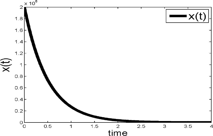
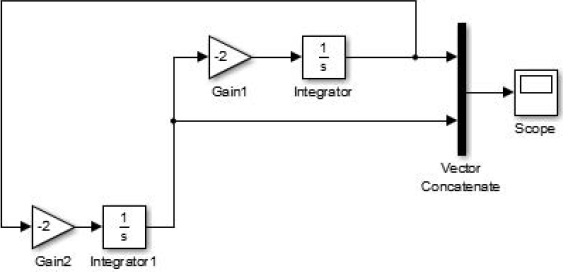
About 70 students (basically the other half), could not find an analytical solution like the one reported in Section 4.1. That is, most of them (49), could identify that model (1), represented the problem at hand, but only 40 of them could find the general solution (10). However, they could not find a particular solution such as (11). These students took a different approach, as they chose to explore a numerical-computational solution for (9, Eq:GeneralAnalitycalSolutions). Some of them implemented code in a software like Matlab or a visual blocks model in Simulink like the one shown in Fig. 3. This time 40 different solutions were obtained like the one shown in Fig. 4.

4.3 Fuzzy Differential Equation Approach
From Sections 4.1 and 4.2 it is clear that 132 students (i.e., 88%) of the students found a solution for the proposed problem. Moreover, 130 different solutions were found. It is important to note that the 130 different solutions were all correct, as the students considered different ways to count the initial population from Fig. 2. But, it is also important to note that 18 students (12%) have not found a solution for the proposed problem.
At this stage, all students were understanding that uncertainty is an important concept to consider in problem solving. So, to this end students were sensitized and focused to learn about fuzzy differential equations, and the following solution was presented.
Model (9), can be considered as the fuzzy differential equation:
where the initial condition
If
First, find the eigenvalues and eigenvectors of the coefficients matrix. The eigenvalues are
Now, the initial condition
If
and the general solution of the system (16) is:
Now, with initial condition
Considering for the specific case of study the fuzzy differential equation (12) with
It is clear that if there is no uncertainty on the initial condition and it is the real number
If
Now the initial conditions
The solution for system (22) is:
If
Now the initial condition is given by
The above analysis concludes the analytical solution for the fuzzy differential equations, and from this analytical solution, students easy built a numerical-computational solution for it. Students easily inferred that for the first form (14), the Simulink model of Fig. 5 is built to compute solutions, and for the second form (17), students built the Simulink model reported in Fig. 6.

All solutions have to be bounded inside curves like those reported in Figs. 7 and 8, for the first and second form respectively. These solutions are considering bound values for
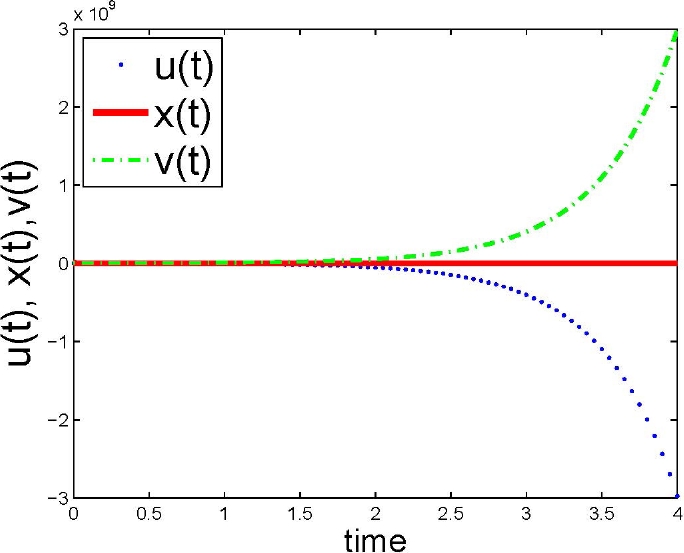

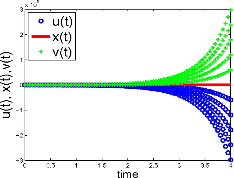
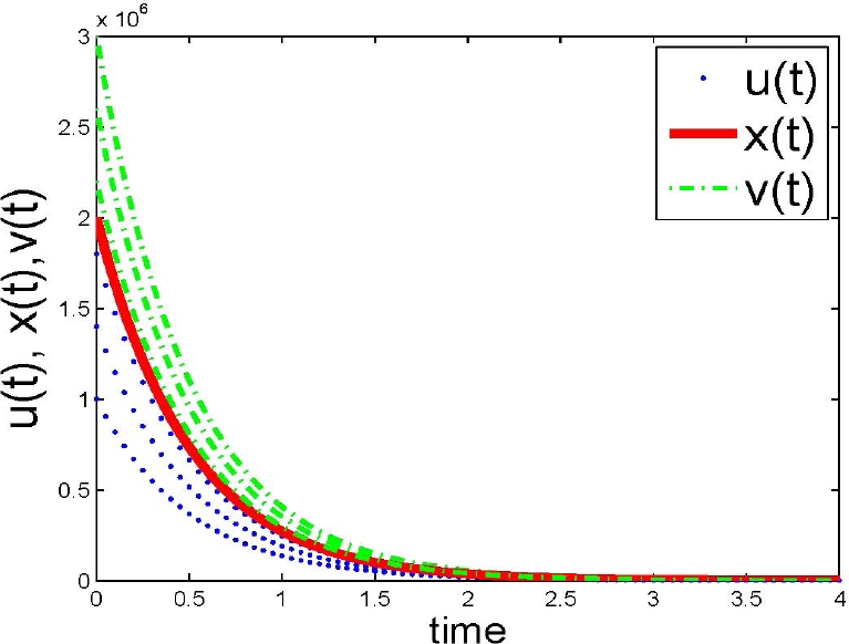
Here, it is important to note that students easily identified from Figs. 7 to 10 that applying the concept of convergence, the desired solution is the one given by the second form, that all solutions are considered in Fig. 10, i.e. Fig. 11 shows 10, but are highlighted solutions for initial conditions of

As a remark, it is important to note that the obtained results allow to predict that the same approach can be considered in other kinds of optimization problems such as time series forecasting, considering the confidence limit like a nested succession with vanishing limit diameter [24].
5 Conclusion and Future Work
Teaching about uncertainty is an important topic that has to be included in engineering and sciences educational programs. Fuzzy differential equations as reported in this paper is an excellent opportunity to introduce this concept, the importance of uncertainty, and finally how to model it.
Problem based learning is an alternative educational strategy to introduce the importance of learning about uncertainty. Moreover, the same didactic resources used to teach about certain phenomenon can be used to improve student skills by exploring the effects in the phenomenon dynamics when the uncertainty is included into the model.
As future work, it is intended to teach problems like control engineering, time series forecasting, economic analysis, etc. Moreover, the application of fuzzy differential equations out of academic environments is considered as a consequence of promoting fuzzy differential equations to be a widely used tool.

