


 text new page (beta)
 English (pdf)
 Article in xml format
 Article references
 Send this article by e-mail
 Cited by SciELO
  Similars in
SciELO
Similars in
SciELO 
 Permalink
1 Introduction
1.1 Background
With the proliferation of mobile devices and advances in wireless communication technologies, mobile ad-hoc networks (MANETs) [24] have drawn the attention of the research community in the last few years. A MANET is a collection of mobile devices, called nodes, such as laptops, smartphones, etc. These nodes are interconnected by wireless links without the aid of any fixed infrastructure or centralized administration.
In MANETs, each node acts both as a host and as a router to forward messages for other nodes that are not within the same radio range. They are free to move and form an arbitrary topology. Then, MANETs are characterized as an extremely dynamic system where links between nodes change over time. A vehicular ad-hoc network (VANET) [5] is an example of a MANET. It is an emerging technology that allows vehicles on roads to communicate for enhancing the driving safety, reducing the congestion, etc.
To model dynamic networks, we use the evolving graph model [15] which consists in recording the evolution of the network topology as a discrete sequence of static graphs. The communication between nodes and the nodes behavior can be modeled by a distributed algorithm [25]. The latter is designed to run on interconnected autonomous computing entities in order to achieve a common task.
To make designing distributed algorithms easier, we use local computation models and particularly graph relabeling systems [23]. A graph relabeling system is based on a set of relabeling rules which are executed locally. These rules, closely related to mathematical and logical formulas, are able to derive the correctness of distributed algorithms.
1.2 Motivation
Proving the correctness of distributed algorithms in dynamic networks represents a non-trivial challenge. In fact, wireless communications need to be taken into account to faithfully specify and verify algorithms requirements. Different approaches have been proposed in the literature in order to redefine distributed algorithms in dynamic networks and prove their correctness [7] [16] [9] [22] [10] [4]. However, the major limitation of the studied works is the lack of consensus about their developments and their proofs. Furthermore, proofs which have been presented are done manually.
In addition, distributed algorithms can be applied only to a particular type of graphs such as tree, ring, etc. In our previous work [14], have adopted the centralised counting algorithm which operates on the star topology. In this paper, we deal with algorithms which operate on a tree-based topology like election and coloration. A tree in a graph is an acyclic and a connected subgraph and a set of disjoint trees is called forest. According to [11], the network can be partitioned anytime into several connected components. Each one represents a given cluster of nodes that evolves semi-independently. In this case, we can talk about a forest of spanning trees, where a spanning tree is formed in every connected component. Previous works [20] demonstrated the validity of using spanning trees in networking area. Indeed, establishing a spanning tree in the network is a well known strategy in communication networks. The availability of such structures can be really useful to simplify a large number of tasks, among which broadcasting, routing or termination detection.
1.3 Contribution
In order to efficiently construct and maintain tree-based topologies, we propose a formal pattern based on the Dynamicity Aware- Graph Relabeling Systems (DA-GRS) model [8]. This model is an extension of graph relabeling systems. To specify our pattern, we use a formal method which provides a real help for expressing correctness with respect to safety properties in the design of distributed algorithms. Our proposed approach is based on the correct-by-construction paradigm [17]. The latter can be supported by a progressive and incremental process controlled by refinement [3] of models for distributed algorithms. This process allows us to simplify the proofs and to validate the integration of requirements. The Event-B formal method [1] can support this methodological proposal suggesting proof-based guidelines. An overview of our proposed approach has been presented in [13].
The main contributions of this paper are as follows:
To propose a formal pattern which allows us to construct and maintain tree-based topologies in dynamic networks based on the DA-GRS model.
To illustrate our proposed pattern by an example of a greedy coloring algorithm of a tree. This algorithm consists of assigning the minimal number of colors which ensures that the color of each node in the tree is different from those of its neighbours. Our approach can guide the user to specify other algorithms which operate on tree-based topologies.
To show the efficiency of our solution in terms of proofs reduction, we present the proof statistics comparing the development of this algorithm with and without using the pattern. So, we can reduce efforts of proofs and specification.
1.4 Organization of the Paper
The paper is organized as follows: Section 2 presents a review of related works. In Section 3, we introduce preliminary notions of the evolving graph model and Event-B formal method. Section 4 provides an informal description of the proposed pattern. In Section 5, we specify our pattern with the Event-B method. Section 6 presents a case study which illustrates the efficiency of our solution. Finally, Section 7 concludes this paper and provides insights for future work.
2 Related Work
Several works have addressed the problem of proving the correctness of distributed algorithms in dynamic networks. In our work, we have reused the framework introduced by A. Casteigts [7], where graph relabeling systems are coupled with evolving graphs. In fact, he proposes an analysis framework for distributed algorithms on dynamic networks. This framework provides general formalisms and methods for studying the main properties of distributed algorithms. It allows to characterize the necessary and/or sufficient connectivity conditions required for the success of a distributed algorithm in dynamic networks. To illustrate it, he analyzes three simple algorithms (propagation algorithm, centralized counting and decentralized counting).
The proposed framework [7] was extended in [22] to provide a sufficient condition for the decentralized counting algorithm. In fact, the author shows that a complete underlying graph is sufficient to prove the correctness for the decentralized counting algorithm. In addition, he introduces the concept of tight conditions to strengthen the guarantees offered by necessary and sufficient conditions. Indeed, a condition is tight if at least one execution sequence of the algorithm over the evolving graph reaches the desired state. Then, he demonstrates the tightness of the sufficient condition provided for the decentralized counting algorithm.
M. Barjon et al. [4] has addressed the construction and the maintenance of a spanning forest (the synchronous case), without any kind of assumption on the rate of changes. The proposed algorithm is the adaptation of a coarse-grain interaction algorithm proposed by A. Casteigts et al. [10] (asynchronous case). It allows the maintenance of a non-minimum spanning forest in unrestricted dynamic networks, using an interaction model inspired from graph relabeling systems. This algorithm is based on token circulation techniques that turn splitting and merging of trees into purely localized phenomena. In fact, a computation step takes as input the state of a pair of nodes and modifies these states according to certain rules.
According to this study, we notice the absence of a general model to specify and prove the correctness of distributed algorithms on evolving graphs. In addition, only [10] and [4] have focused on the forest topology. Furthermore, proofs which have been presented are done manually.
3 Basic Concepts
In this section, we provide some basic concepts to explain our work. First, we present the evolving graph model to record the dynamic behavior of a network topology. After that, we give an overview of the Event-B method.
3.1 Evolving Graph Model
The evolving graph model, proposed in [15], represents
an abstraction of dynamic networks, through the formalisation of a time domain
in graphs. In this model, a dynamic graph can be decomposed as a sequence of
static graphs. Each static graph represents a snapshot of the dynamic network at
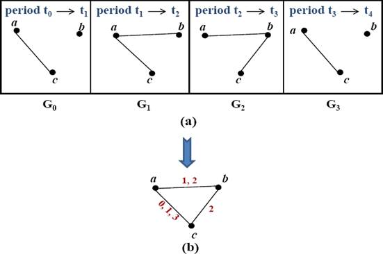
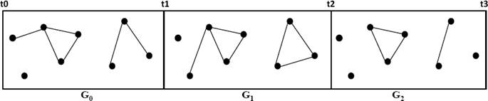
a given time. As an example, we consider the four snapshots taken at different
time intervals of a MANET, as depicted in Fig.
1. Formally, let S𝕋 =
t0, t1, ...,
tn be a sequence of increasing dates used to
capture static graphs. These dates correspond to every time step in a
discrete-time system ( ). Except for
t0 and tn, each
ti corresponds to one or more topological
events that modify the network. Let SG =
G0, G1, ...,
Gn-1be the sequence of
undirected static graphs. Each Gi represents the
network topology during the period [ti,
ti-1) in the evolving graph
g. Finally, let Gi be the union
of all Gi in SG, called
the underlying graph of g (see Fig. 1 (b)). The edges are labeled with the date of their presence.
For example, the presence of the edge “ab” in Fig. 1(a) at the dates “1” and “2” is
represented in Fig. 1(b) by an edge
“ab” labeled “1, 2”. Then, the triple
g=(G, SG,
S𝕋) is the corresponding evolving
graph.
). Except for
t0 and tn, each
ti corresponds to one or more topological
events that modify the network. Let SG =
G0, G1, ...,
Gn-1be the sequence of
undirected static graphs. Each Gi represents the
network topology during the period [ti,
ti-1) in the evolving graph
g. Finally, let Gi be the union
of all Gi in SG, called
the underlying graph of g (see Fig. 1 (b)). The edges are labeled with the date of their presence.
For example, the presence of the edge “ab” in Fig. 1(a) at the dates “1” and “2” is
represented in Fig. 1(b) by an edge
“ab” labeled “1, 2”. Then, the triple
g=(G, SG,
S𝕋) is the corresponding evolving
graph.
3.2 Event-B Overview
The Event-B modeling language is an evolution of the B language [1]. A system specification (model) in Event-B consists of two types of components: context and machine.
Context. A context specifies the static parts of a model. It may contain carrier sets, constants, axioms, and theorems that can be derived from the axioms of a context.
Machine. An Event-B machine describes a reactive system. It may contain variables, invariants, theorems, and events. Variables define the state of a machine. They are constrained by invariants. An invariant is defined to be a predicate preserved by each event. The dynamic behavior of the system is defined by the set of events specified in the Events clause. Generally, an event can be defined as follows:

where: Pr is a set of parameters, G is the guards which specify the necessary conditions for the event observation, S is the action which consists in several assignments. The assignments can be either deterministic or non-deterministic. A deterministic assignment has the standard syntax and meaning. It is denoted by x:= E(k, v) where x is a state variable and E(k, v) is an expression.
A non-deterministic assignment can be of two forms: (a) The first form, x :∈ E(k, υ), arbitrarily chooses a value from the set E(k, v) to assign to x. (b) The second form is denoted by x : |Q(x, y, x') which arbitrarily chooses to assign to x a value that satisfies the predicate Q. Q is called a before-after predicate and expresses the relation between the previous values x (before the action) and the new ones x’ (afterwards).
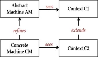
Refinement. The concept of refinement is the main feature of Event-B. The refinement of a machine allows to enrich it in a step-by-step fashion. It is the foundation of the correct-by-construction approach [17]. It is also used to transform an abstract model into a more concrete version by modifying the state definition. In fact, new variables and events can be introduced. Furthermore, abstract events can be refined to more concrete ones. The relation between variables in the concrete and abstract model is given by a gluing invariant. The relationship between machines and contexts is defined as shown in Fig. 2: A machine AM may see a context C1, this means that all carrier sets and constants defined in C1 can be used in AM. A machine CM can be built to be a refinement of the machine AM. CM is called a refinement or a concrete version of the machine AM. Likewise, a context C2 can extend the context C1, this means that all properties defined in C2 are added to C1.
Proof Obligations. An Event-B specification is considered as correct only if each machine, as well as the process of refinement, is proved by adequate Proof Obligations (POs); i.e events preserve the invariant(s) and each event is feasible. POs are generated by the RODIN tool [2], which provides an environment for developing correct-by-construction models for software-based systems. They can be discharged either automatically by an integrated proof tool or through interactive proof tool.
4 Informal Pattern Presentation
In software engineering, the idea of design patterns [19] is to have a general and reusable solution to commonly occurring problems. In general, a design pattern is not necessarily a finished product, but rather a template on how to solve a problem which can be used in many different situations. In this section, we propose a formal pattern for specifying and proving the correctness of distributed algorithms in dynamic networks. It can be applied only to algorithms which operate on a tree-based topology. The proposed pattern defines the different topological changes in a dynamic network and the manner of time evolution. Let g = (G, SG, S𝕋) be an evolving graph. Every static graph, Gi ∈ SG, corresponds to the network topology during the interval of time [ti, ti-1) where ti represents the date when one or several topological events occur in the system. In this paper, we take into consideration only the appearance and disappearance of edges in the network like the existing works in this context [10] [4] [7] [22]. Then, we can distinguish two events:
Adding edge: It consists in adding a new edge to the graph at the current date t.
Removing edge: It consists in removing an edge from the graph at the current date t.
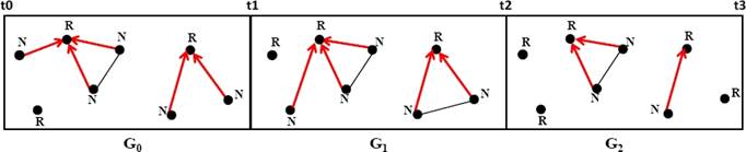
In order to efficiently construct and maintain tree-based topologies, we use the DA-GRS. The latter is a local computation based model which guarantees that the network remains covered by a spanning forest at any time, in which 1) no cycle can possibly occur, 2) every node belongs to a tree (an isolated node belongs to a tree with a single node which is the root) and 3) there is always exactly one root (also called token) in every tree.
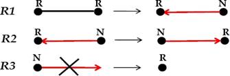
The root of each tree is labeled R and the other nodes are labeled N. The DA-GRS is based on three rules which are presented in Fig. 3:
R1: Merging rule. Whenever two tokens (nodes labeled R) arrive at the endpoints of the same edge, one of them destroys its token and selects the other as parent. As a result of this rule, the two trees merge.
R2: Circulation rule. If there is no possible merging, a node in the state R (has the token) passes the token to one of its neighbours in the tree (child) which becomes the new root.
R3: Regeneration rule. Whenever an edge of the tree disappears, the node on the child side (labeled N) does not possess the token. In this case, there will exist a tree without a token. Then, the node must regenerate a token (i.e. it becomes a root).
In this work, we assume that the incrementation of time from a date t to a date t+1 is done after: 1) at least one appearance and/or disappearance of an edge is performed in the network and 2) each connected component of the network is covered by a spanning tree.
5 Formal Development of the Pattern
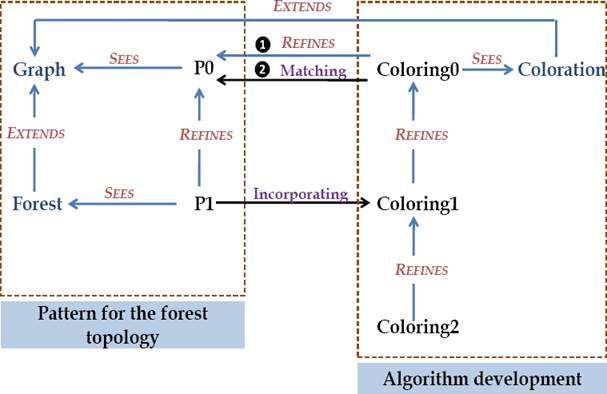
As mentioned earlier, the specification of our pattern is performed with the Event-B method and done with the RODIN platform. An Event-B development is an incremental process controlled by the refinement of models. We note that two basic levels are necessary to build a correct pattern as shown in Fig. 4.
The first model P0: We can notice only the appearance of new edges and disappearance of other edges from a graph Gi at a date ti to the following graph Gi+1 at a date ti+1 (see Fig. 5). The system time is initialized to zero (t=0).
At this date, no topological event (events which modify the topology) has been performed. The incrementation of time is done, if one or several topological events (add edge and/or remove edge) have been produced. Formally, we define three events:
Add_Edge: This event is observed when an edge does not belong to the graph at a current date t. As a result, this edge will be added to the graph.
Remove_Edge: It consists in removing an existing edge of the graph at a current date t.
Increment_Time: This event is observed when one or several topological events (Add_Edge and/or Remove_Edge) occur in the network.
The second model P1: Once the machine of the first level has been specified and proven, it can be refined in order to build and maintain a forest of spanning trees in dynamic networks. In fact, we introduce labels of nodes to specify the DA-GRS rules. Formally, we add three events (Merging_Rule, Regeneration_Rule and Circulation_Rule) and we refine the events specified in P0 to take into consideration the local label modification. At this level, we indicate that the incrementation of time can take place, if each connected component of the network is covered by a spanning tree.
In fact, we suppose that the algorithm for building and maintaining a spanning forest (DA-GRS rules) acts as an “observer” that knows when a spanning tree is formed in each component. This kind of detection is called observed termination detection [18].
An example of the evolving graph sequence, which refines the first level, is shown in Fig. 6. In this figure, a spanning tree in each component is presented with red color. The nodes which do not belong to any tree edge (isolated nodes) are labeled R. In fact, every node forms a tree of its own and is the root of that tree (it has a token).
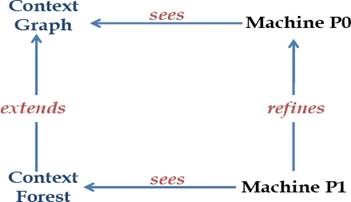
With these machines, contexts are required with a particular definition in the specification. The first one is the context Graph which defines the basic properties of the network. The second one is the context Forest. It is defined as an extension of the context Graph. It specifies elements of a tree and includes node labels that describe the DA-GRS rules.
5.1 Formal Specification of the Contexts of the Pattern
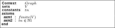
The context Graph: A graph is modeled by a set of nodes called V. In our work, we have supposed that a dynamic graph is composed of stable nodes. For this reason, we define V in the context as an abstract set. Listing 1 shows the specification of the context Graph. By means of the axm1, we specify that the number of nodes in the network is finite. Moreover, we introduce a constant, called tn, which represents the final system date. This constant is an integer different to the start date of the system (see axm2).
The context Forest: A tree can be defined as an acyclic and connected subgraph. In order to specify a tree, we have to define a node r (r ∈ V1 and V1 ⊆ V) which is the root of the tree and a parent function t (see Listing 2). Otherwise, each node has a unique parent node, except for the root. For more information about tree building, the reader can read [6]. Formally, we obtain the following Event-B definition: t ∈ V1 \ {r} → V1. A tree is an acyclic subgraph. A cycle c in a finite graph t built on a set V1 is a subset of V whose elements are members of the inverse image of c under t, formally: c ⊆ t−1[c].
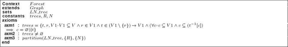
In order to guarantee the non existence of a cycle in a tree, we must prove that the set c is equal to the empty set. As in [6], we describe this property in the following way: ∀c · (c ⊆ V1 ∧ c ⊆ t−1[c]) ⇒ c = ∅.
We introduce the constant trees to be the set of all trees (with root r) of the graph g. Also, we add some requirement properties: trees is non-empty set of possible trees on the graph (axm2) and each node is labeled R or N (axm3). We specify label nodes as a set called LN_tree.
5.2 Formal Specification of the Machines of the Pattern
The initial model (Machine P0): At this abstract level, we define the machine P0 which sees the context Graph. The invariants specification of P0 is given in Listing 3. At a current date t, a network can be formally modeled as a simple and undirected graph g where nodes denote processors and edges denote direct communication links (inv1). An undirected graph means that there is no distinction between two nodes associated with each edge (inv2).
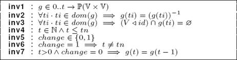
A graph is simple, if it has zero or one edge between any two nodes and no edge starts and ends at the same node (inv3). The domain restriction “V ◁ id” is a subset of the relation id that contains all of the pairs whose first element is in V. The identity relation “id” maps every element to itself.
The current date t is an integer lower or equal to the final system date (inv4). Moreover, we introduce a new variable called “change” (inv5). If one topological event has been produced, “change” is set to “1”, otherwise “change” is set to “0”. So, if “change” is equal to “1”, the date t is different from the final date tn (inv6). By means of the invariant inv7, we specify that if the current date t is strictly greater than “0” and “change” is equal to “0”, then the graph does not undergo any topological event (g(t)=g(t-1)).
Initially, the system date is equal to zero (t = 0). Also, the variable “change” is equal to zero which means that no topological event has been produced. At this abstract level, we define three events:
Event Add_Edge: This event, specified in Listing 4, is activated when an edge “x ↦ y” between the nodes x and y does not belong to the graph g at the current date t(grd1, grd2 and grd3) and “t” is different to the final date “tn” (grd4). As a result, this edge will be added to g(t). To respect the invariant inv2, we add both “x ↦ y” and “y ↦ x” to g(t) (act1). Also, the variable “change” takes the value “1” (act2) to indicate that a topological event has been produced.

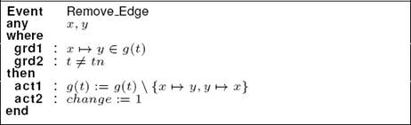
Event Remove_Edge: As depicted in Listing 5, an edge has been removed at the current date t if it is present in the graph (grd1) and “t” is different to the final date “tn” (grd2). In the action component, we update the graph g(t) (act1) and we set the variable “change” to “1” (act2).
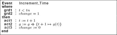
Event Increment_Time: This event (see Listing 6) can be triggered if one or several topological events have been produced. In the guard component, we verify that the current date t is strictly lower than the final system date tn (grd1) and the variable “change” is equal to “1” (grd2). In the action component, we increment the time to “t+1” and we set the graph at the date “t+1” to the graph g(t) (act1 and act2). In addition, we reset the variable “change” (act3). So, we have no topological change at the date t +1.
The second model (Machine P1): To specify the machine P1, we begin by adding two variables:

The addition of these two variables involves adding new properties. We have formalized these properties in the form of Event-B invariants as follows:
-
There is no intersection between the nodes of the disjoint trees: This constraint is ensured by the invariant inv3. We note that the domain of tr1 (dom(tr1)) is the set of the first parts of all the pairs of nodes in tr1. Also, the range of tr1 (ran(tr1)) is the set of the second parts of all the pairs of nodes in tr1.
inv3: ∀ti, tr1, tr2·ti ∈ dom(Trees t) ∧ tr1 6= tr2 ⇒ (dom(tr1) ∪ ran(tr1)) ∩ (dom(tr2) ∪ ran(tr2)) = ∅
-
Each disjoint tree has only one root labeled R and all the other nodes are labeled N.
inv4: ∀ti, tr·ti ∈ dom(Trees t)∧tr ∈ Trees t(ti) ⇒ (∃x·(x ↦ti) ∈ dom(lab) ∧ lab(x ↦ti) = R ∧ (∀y·y ∈ (dom(tr) ∪ ran(tr)) \ {x} ∧ (y ↦ ti) ∈ dom(lab) ⇒ lab(y ↦ti) = N))
-
A node which does not belong to any disjoint tree (it can belong to graph edges) is labeled R. It forms a tree of its own and it is the root of this tree.
inv5: ∀ti, x·ti ∈ dom(Trees t) ∧ x ∈ V ∧ ({{x}} ∩ {tr.tr ∈ Trees_t(ti)|dom(tr) ∪ ran(tr)} = Ø) ⇒ lab(x ↦ ti) = R
Initially, all the nodes are labeled R at the date “t=0”. Otherwise, every node is considered as a tree with a single node and it is the root of this tree. Then, the set of disjoint trees is empty (Trees_t(0)= ∅).
In order to construct and maintain tree-based topologies:
We introduce three events: Merging_Rule, Regeneration_Rule and Circulation_Rule.
We refine the events of P0 in order to take into consideration local label modification.
In this paper, we only detail the specification of the refined events of P0.
Specification of the event Add_Edge: At this second level, the event Add_Edge presented in the machine P0 remains unchanged. In fact, the appearance of a new edge in the network at the current date t requires only the addition of the edge, without modifying the labels of nodes.
Specification of the event Remove_Edge: We refine the event i detailed at the first level by reinforcing the guard component. In fact, we add a new guard (grd3: ∀tr·t ∈ dom(Trees_t) ∧ tr ∈ Trees_t(t) ⇒ (x ↦ y ∉ tr ∧ y ↦ x ∉ tr) to specify that the removed edge (x ↦ y and y ↦ x) does not belong to any disjoint tree at the current date t.
Specification of the event Increment_Time: We refine the event Increment_Time presented in the machine P0 as depicted in Listing 8. In fact, we add a new guard grd3 to indicate that each connected component at the date t is covered by a spanning tree.

Then, two neighboring nodes x and y of the graph should belong to the same spanning tree. In the action component, we add two actions (act4 and act5) to indicate that the set of disjoint trees at the date t+1 is equal to Trees_t(t) (act4). Moreover, the labels of nodes at the date t+1 are equal to the current labels at the date t (act5).
6 Case Study: Tree-coloring Algorithm
To illustrate the proposed pattern, we present the greedy coloring algorithm which operates on tree-based topologies, encoded by the local computations model. This algorithm is used in many practical applications such as scheduling [21] and register allocation in compilers [12].
The main objective of this section is to demonstrate how the pattern can be used and incorporated during development to specify the coloring algorithm. Firstly, we present an overview of the coloring algorithm. Secondly, we explain how we can use our pattern to specify the algorithm. Thirdly, we detail the specification of the algorithm. Finally, we illustrate the efficiency of our solution by comparing the proof statistics of this algorithm with and without using the pattern.
6.1 Algorithm Overview
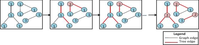
Let’s consider a tree with a degree equal to D. We suppose that the number of colors is equal or less than “D+1”. The set of colors are identified by the numbers (1,..., D+1). Initially, all the nodes are colored by the color number “1” in the colors list. The coloring algorithm is given by the rule R presented in Fig. 7. It can apply a computation to a star. A star is a node with its neighbours.

If the node (center) has the same color (Ci) as one of its neighbours, it changes its color with a new color C’. The number associated with the color C’ is equal to “max(C1, Ci, Ck)+1”. That is to say, it takes the lowest color value which is different to all the neighbours colors of the center node.
A run of the algorithm consists in applying the relabeling rule R specified by the algorithm until this rule becomes not applicable. In the final configuration, all the adjacent nodes in the tree have different colors.
6.2 Using our Pattern in the Development of the Tree-coloring Algorithm
In this section, we present the idea of the pattern incorporation into an Event-B development. In fact, we explain how our pattern is used to correctly specify the tree-coloring algorithm. The process can be seen in Fig. 8.
Generally, the development of a distributed algorithm in Event-B starts with a very abstract model. Then, by successive refinements, we obtain a concrete one that expresses the local behavior of processors in the network. Each refinement level is defined by an Event-B machine. We follow the different steps to refine and incorporate the proposed pattern during the system development:
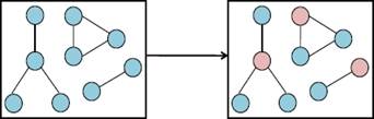
Step 1: We define a machine Coloring0 which refines the machine P0 (❶ in Fig. 8). Then, it includes the events of P0. We have to add one event (oneshot) which specifies the result of the algorithm in one shot and does not describe how the solution is computed. The analogy of someone closing and opening their eyes. This level can verify that a colored graph can be obtained from an initial graph where all the nodes have the same color. In the colored graph, we can notice that, in each connected component, the center of each star has a color different to at least one of its neighbours (see Fig. 9).
To specify the machine Coloring0, we need to add a new context called Coloration to specify algorithm properties. Coloring0 can access to all components of the context Graph via the clause “SEES”.
Step 2: In order to specify the machine Coloring1, we use the approach proposed by T. Hoang et al. [19] for reusing existing patterns in Event-B. Concretely, we use a tool, as a plug-in for the RODIN platform, provided by T. Hoang et al. In fact, we match all variables, events and context information of the pattern specification P0 with those of the machine Coloring0 (❷ in Figure 8). Then, the refinement P1 can be incorporated to create the refinement Coloring1 of Coloring0. The generated refinement is correct-by-construction and no proof obligation needs to be generated. For more details about the methodology proposed by T. Hoang et al., the reader can see [19]. In the machine Coloring1, we add some details to globally specify the computation of the algorithm result. In fact, we refine the event introduced at the first level to ensure that each connected component is covered by a spanning tree. Also, each pair of neighbouring nodes of a spanning tree do not share the same color (see Fig. 10). Moreover, we introduce a new event to ensure the graph coloration.
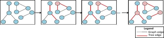
Step 3: We introduce a new machine called Coloring2 which refines Coloring1. Coloring2 specifies locally the nodes interactions in order to correctly color the nodes of each connected component (spanning tree) in the graph. It is an application of the relabeling rule R (see Fig. 11).
6.3 Formal Specification of the Tree-coloring Algorithm
6.3.1 The Context Coloration
To specify the coloring algorithm, we add a new context called “Coloration” (see Listing 9) which extends the context “Graph”. We define “colors_list” as a finite set of colors (axm1). The cardinality of “colors_list” is less than card(V) (axm2). Let’s “color” be a constant defined by the axiom axm4. It is a bijective function which assigns a unique color to each identifier.

6.3.2 The First Level: Machine Coloring0
The machine Coloring0 refines the machine P0 of the pattern. At this abstract level, Coloring0 expresses only the goal of the distributed algorithm and does not describe the process of computing the solution. Formally, the events Add_Edge and Remove_Edge remain unchanged and we add one new event called “oneshot”.
To specify this event, we need to introduce some variables (see Listing 10):
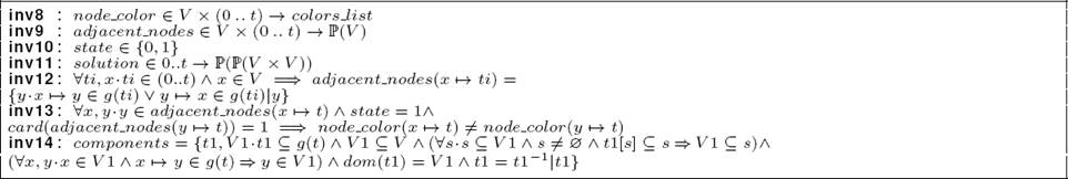
— nodes_color: It contains the color of each node in the graph at the current date t. Formally, this variable is specified in inv8 of Listing 10. Initially, at the date “t=0”, all the nodes have the same color.
— adjacent_nodes: It assigns to each node at a date from (0..t) the set of its neighbouring nodes (inv9).
— state: It allows to check if the system reaches a stable state. In fact, if the event oneshot is triggered, the variable “state” takes the value “1” otherwise “state” is equal to “0” (inv10). Initially, this variable is equal to zero. If “state” is equal to “1”, only the event Increment_Time can be activated.
— solution: It contains the set of colored and connected components at the current date t (inv11). Initially, all the nodes have the same color. Then, solution(t) is empty.
— components: It specifies the set of connected components in the graph at the current date t (inv14).
The addition of these variables requires adding other properties in the invariant component as depicted in Listing 10:
— The set of neighbors of a node “x” at a date ti is the set of nodes that are connected to “x” in the graph g(ti) (inv12).
— If the variable “state” is equal to “1”, each node having the degree “1” has a color different to its neighbor (inv13).
Specification of the event oneshot
At the first level, the event oneshot reveals the result of the coloring algorithm in one step without describing how the solution is computed. It verifies that, in each connected component, each node has a color different to at least one of its neighbours. In Listing 11, we provide the specification of the event oneshot.

In the guard component, we verify some constraints:
— The parameter “colored_components” is a set of colored and connected components in the graph (grd1).
— The set of connected and colored components at the current date t is empty (grd2).
— There is no intersection between the nodes of colored_components (grd3).
— Each edge in the graph I(t) is an edge of a colored and connected component (grd4).
— Each node, which is adjacent to a node of a connected component, must belong to this component (grd5).
— Each node of colored_components has a color different to at least one of its neighbours (grd6).
— The system does not reach a stable state and the date t is strictly lower than “tn” (grd7).
— One or several topological events have been produced in the graph (grd8).
In the action component, we specify that “Solution(t)” contains the set of colored and connected components (act1). Moreover, we set the variable “state” to “1” (act2).
At this level, we reinforce the event Increment_Time of the pattern as shown in Listing 12.
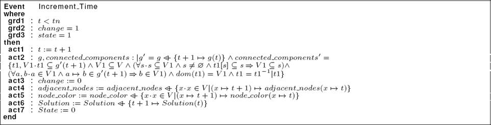
In fact, we add a new guard grd3 to verify that the system reaches a stable state. Otherwise, the event Increment_Time can be activated only if “state” is equal to “1”. Moreover, we reinforce the action component to reinitialize the set of adjacent nodes, the color of each node and the solution of the algorithm at the date t+1 (act4, act5 and act6). Also, we update the variables State and connected_components to “0” (act2 and act7).
In order to prohibit the triggering of topological events after the event oneshot, we reinforce the events Add_Edge and Remove_Edge by adding a new guard (state=0).
We present in Fig. 12 the sequencing between the events of the machine Coloring0. The diagram explicitly illustrates that after the initialization of all the machine variables, one or several topological events can be triggered using the event Add_Edge or Remove_Edge.
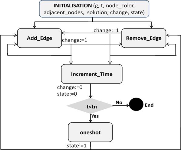
The consequence of the events occurrence may allow the triggering of the event Increment_Time followed by the event oneshot if the actual date is lower than the final system date. The event oneshot is followed either by Add_Edge or Remove_Edge events.
6.3.3 The Second Level: Machine Coloring1
The refinement of Coloring0 named Coloring1 introduces more details about the coloring algorithm. At this level, we can notice at a current date t a forest of spanning trees, where a spanning tree is formed in every connected component. In each spanning tree, each pair of adjacent nodes have different colors.
The specification presented at the first level of the pattern still exists. However, we have to add a new property in the invariant component. It specifies that when the system reaches a stable state (state=1), each two adjacent nodes in a disjoint tree have different colors:
∀ti, x, y·ti ∈ (0..t) ∧ tr ∈ Trees t(ti) ∧ x ∈ (dom(tr) ∪ ran(tr)) ∧ y ∈ adjacent nodes(x ↦ti) ∧ state = 1 ⇒ y ∈ (dom(tr) ∪ ran(tr)) ∧ node_color(x ↦ti) ≠ node color(y ↦ ti)
At this level, we refine the event oneshot defined in Coloring0. Indeed, we have to reinforce the guard component to verify some constraints (see Listing 13):
Each connected component at the date t is covered by a spanning tree. Then, two neighbouring nodes x and y of the graph should belong to the same spanning tree (grd1).
The set of colored and disjoint trees at the date t is empty (grd2).
All adjacent nodes in each disjoint tree do not share the same color (grd3).

The abstract parameter “colored_components”, defined in the machine Coloring0, is replaced with concrete value by means of a witness. In fact, “colored_components” represents at this level the set of disjoint trees. In Event-B, a witness is defined as a simple equality predicate involving the abstract parameters.
In the action component, we reinforce the action act1 to specify that “solution(t)” is equal to the set of disjoint trees at the date t.
In order to ensure the graph coloration, we introduce the event “Progress” as shown in Listing 14. In the guard component, we define tr as a disjoint tree at the date t (grd1). The nodes x and y are two adjacent nodes of the tree tr (grd2 and grd3). By means of the guard grd4, we specify that x and y have the same color. The parameter “c” represents a color different to the color of the nodes x and y (grd5). In the guard grd6, we verify that “state” is equal to “0” and the date “t” is lower than “tn”. In the action component, we update the color of the node x to “c” (act1).
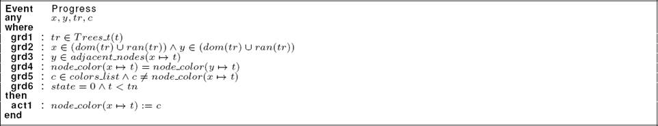
Fig. 13 depicts the sequencing between the events of the machine Coloring1. Initializing the variables of the machine may allow the triggering of the event Add_Edge, Remove_Edge or the merging of two disjoint trees by the event Merging_Rule. These three events are followed by the event Increment_Time if one or several topological events have been performed (change=1).
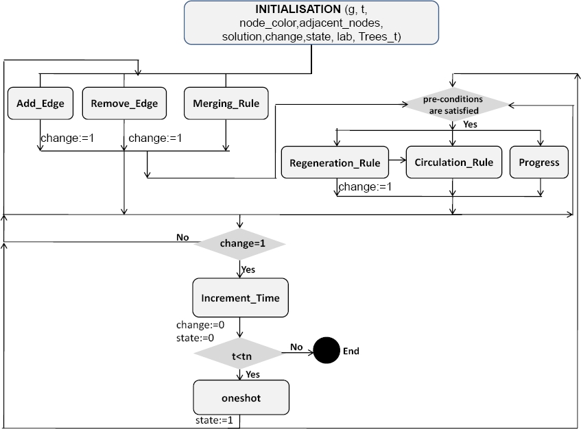
The occurrence of these events can be also followed by the event Regeneration_Rule, Circulation_Rule or Progress if the corresponding pre-conditions (guards) are satisfied. The triggering of the event Increment_Time is followed by the event oneshot if the actual date “t” is lower than the final system date “tn”.
6.3.4 The Third Level: Machine Coloring2
The third machine, called Coloring2, refines the previous one (Coloring1) to describe the local label modification and encode the relabeling rule described in Fig. 7. Formally, we introduce four variables in the machine Coloring2:
-
degree_node: It is defined as a total function which indicates the degree of each node in a disjoint tree at a date from (0..t). Initially, the degree of each node in a tree is equal to the cardinality of its neighbours which belong to this tree.
inv1: degree node ∈ (V × (0..t)) → ℕ.
-
trees_at_ti: It is defined as a total function which assigns for each date from (0..t) a set of trees.
inv2:: trees_at_ti ∈ (0..t) → ℙ(trees)
-
degree_tree: It is defined as a total function to specify the degree of a tree at a date from (0..t).
inv3:: degree tree ∈ (tree × (0..t)) → ℕ.
-
colors_for_tree: It is a function which gives the colors of a tree at a date from (0..t).
inv4:: colors for tree ∈ (tree × (0..t)) → ℙ(colors list).
At this level, we initialize the node_color of each node to color(1) which represents the color number “1”. The addition of the four variables involves adding new properties. To do so, we introduce some invariants called gluing invariants which link the abstract state variables to the concrete ones:
-
A tree tr having all the edges included in g(ti) forms a tree at the date ti.
inv5: ∀ti, tr · ti ∈ (0..t) ∧ tr ∈ tree ∧ tr ⊆ g(ti) ⇒ tr ∈ trees_at_ti(ti)
-
All the edges of a tree tr at a date ti are included in the graph g at the date ti.
inv6: ∀ti, tr · ti ∈ (0..t) ∧ tr ∈ trees_at_ti(ti) ⇒ tr ∈ tree ∧ tr ⊆ g(ti)
-
The degree of a node x in a disjoint tree tr at a date ti is equal to the cardinality of its neighbours which belong to tr.
inv7:: ∀ti · ti ∈ (0..t) ∧ tr ∈ Trees t(ti) ∧ x ∈ (dom(tr) ∪ ran(tr)) ⇒ degree(x ↦ti) = card({u · (u ↦x ∈ tr ∨ x ↦ u ∈ tr)|u})
-
At a date ti, a node x which does not belong to any disjoint tree has a degree equal to zero.
inv8:: ∀ti, x·ti ∈ dom(Trees t) ∧ x ∈ V ∧ ({{x}} ∩ {tr.tr ∈ Trees_t(ti)|dom(tr) ∪ ran(tr)} = ∅) ⇒ degree node(k ↦ ti) = 0
-
The degree of a tree tr, at a date ti, is equal to the maximum degree of all its nodes.
inv9:: ∀ti, tr · ti ∈ (0..t) ∧ tr ∈ trees_at_ti(ti) ⇒degree(dom(tr) ∪ ran(tr)) ⇒ degree node(z ↦ti) ≥ 1 tree(tr ↦ ti) = max({x · x ∈ (dom(tr) ∪ ran(tr))|degree node(x ↦ti)})
-
The colors of nodes in a disjoint tree are included in the set of colors “(1..(degree_tree(tr ↦ti) + 1))”.
inv10:: ∀ti, tr · ti ∈ (0..t) ∧ tr ∈ Trees_t(ti) ⇒colors_for tree(tr ↦ ti) ⊆ {i · i ∈ 1..(degree tree(tr ↦ ti) + 1)|color(i)}
-
The color of each node x in a disjoint tree tr, at a date ti, belongs to the set of colors “colors_for_tree(tr ↦ti)”.
inv11:: ∀ti, tr, x·ti ∈ (0..t)∧tr ∈ Trees_t(ti)∧x ∈ (dom(tr)∪ ran(tr)) ⇒ node color(x ↦ ti) ∈ colors_for_tree(tr ↦ ti)
-
We ensure by means of the theorem Th1 that the degree of each tree is lower than the number of all the nodes.
Th1:: ∀ti, tr · ti ∈ (0..t) ∧ tr ∈ trees_at_ti(ti) ⇒ degree_tree(tr ↦ti) < card(V)
-
We verify by means of the theorem Th2 that the degree of each tree node is equal or greater than “1”.
Th2:: ∀ti, tr, z · ti ∈ (0..t) ∧ tr ∈ trees_at_ti(ti) ∧ z ∈ dom(tr)∪ ran(tr)) ⇒ node color(x ↦ ti)≥1
The machine Coloring2 specifies the local label modification and encode the relabeling rule of the algorithm. At every time, each node is in a particular state and this state will be encoded by a node label. According to its own state and to the states of its neighbours, each node may decide to perform a computation step by applying the relabeling rule R. In order to specify the rule R, we introduce a new event called “Rule” depicted in Listing 15.
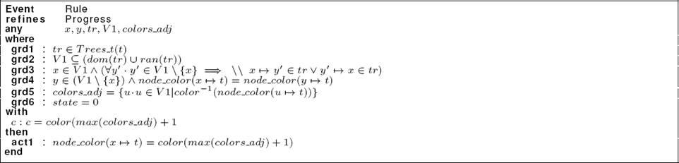
This event refines the event Progress defined in the machine Coloring1. In fact, we reinforce the event Progress by adding two parameters “V1” and “colors_adj”. “V1” is a subset of nodes of the tree tr (grd2) and “colors_adj” represents the colors of all the nodes of V1 (grd5). By means of the guard grd3, we specify that V1 is composed of the node “x” and all its neighbours. We introduce the witness “c: c = color(max(colors adj) + 1)” to replace the abstract parameter “c”, with the color having the number “max(colors adj)+ 1”. In the action component, we reinforce the action act1 to specify that the node x takes the color identified by the number “(max(colors_adj) + 1)”.
At this level, we refine the event oneshot defined in the machine Coloring1 to verify other properties at the end of the algorithm execution (see Listing 16). To do so, we reinforce the guard component. In fact, we add a new guard grd9 to ensure that each node of a disjoint tree has a color identified by the number “1” or “2”. Otherwise, the graph is colored by two colors. We introduce the guard grd10 to specify that all the isolated nodes have the color number “1”. Finally, we refine the event Increment_Time of the machine Coloring1. In fact, we reinitialize the variables degree node, tree at the date t+1. The machine Coloring2 has the same diagram as the machine Coloring1 (see Fig. 13). However, we replace the event Progress by the concrete event Rule.

6.4 What we Gain with the Pattern Approach
One of our objectives in this paper is to reduce the proof efforts. In fact, we aim to increase automatic proofs and decrease those that need interactive efforts to be discharged. Table 1 shows the proof statistics related to the development of the pattern and the coloring algorithm with and without using the pattern.
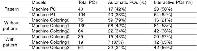
It includes the proof obligations generated and discharged by the RODIN platform and those interactively proved. As we can see, by developing the pattern separately, we have to prove 144 obligations. But we have the following advantages:
We have a significant reduction of the proofs interactively discharged in the machine Coloring0 because Coloring0 is a refinement of P0.
We do not need to prove that Coloring1 is a refinement of Coloring0 since it is correct by construction. In fact, we have already done this proof when developing the pattern. We have to prove only some details related to the tree-coloring algorithm (20 obligations).
We can reuse the pattern to specify other case studies such as election algorithm.
Consequently, we can save efforts on modeling as well as proving the correctness of distributed algorithms in a forest.
7 Conclusion and Future Work
In this paper, we have presented a reuse-based solution for specifying and proving distributed algorithms which operate on tree-based topologies.
Our contribution consists in proposing a formal pattern based on the evolving graph model. It relies on the DA-GRS to construct and maintain a forest of spanning trees in dynamic networks.
To illustrate our pattern, we have presented the tree-coloring algorithm as a case study. The proof statistics show that our solution can save efforts on specifying as well as proving the correctness of distributed algorithms in a forest topology.
As a future work, we plan to illustrate the proposed pattern with other examples of distributed algorithms. We also aim to extend our pattern in order to take into consideration the appearance and disappearance of nodes in the network.
Another direction for future work consists in dealing with other algorithms which operate on other network topologies such as complete graph, ring, etc.

