


Serviços Personalizados
Journal
Artigo
 texto em
  Inglês (pdf)
 Artigo em XML
 Referências do artigo
 Enviar este artigo por email
Indicadores
-
 Citado por SciELO
 -
 Acessos
Links relacionados
-
 Similares em
SciELO
Similares em
SciELO
Compartilhar

 Permalink
Agrociencia
versão On-line ISSN 2521-9766versão impressa ISSN 1405-3195
Agrociencia vol.52 no.7 Texcoco Out./Nov. 2018
Water-Soil-Climate
Fitting with mobile L moments of the GEV distribution with variable location and scale parameters
1 Facultad de Ingeniería de la Universidad Autónoma de San Luis Potosí. Genaro Codina No. 240. 78280 San Luis Potosí, San Luis Potosí. (campos_aranda@hotmail.com)
The frequency analysis of annual maximum hydrological data as floods, intensity of rainfall, sea level, wind speeds and daily maximum precipitation, considers that their records are integrated by independent values generated by a stationary random process; because of this, their properties do not change over time. The construction of reservoirs, the effects of urbanization in the basins and the impact of regional climate change result in annual maximum hydrological data series with trends and non-constant variability that make them non-stationary. The objective of this study was to expose the method of mobile L-moments, to estimate the parameters of location (u) and scale (a) variables with time, used as a covariate in the probability distribution function General Extreme Values of type non-stationary (GVE11), with constant shape parameter (km). Through linear or exponential functions, the variation in time of the parameters u and a was plotted to make predictions that are associated with certain probabilities of non-exceedance in the future (years 2050 or 2100). Based on the standard error of fit, the GVE11 distribution was accepted or rejected as a probabilistic model of large series of extreme hydrological data that exhibit non-constant trend and variability. By means of two numerical applications, the practical approach of the mobile L-moments method was shown and, through predictions for the future, its importance and usefulness were highlighted in the probabilistic analyses of large, non-stationary records of the aforementioned type (with non-constant tendency and variability).
Key words: stationary and non-stationary GVE distributions; linear trend; variability with respect to the mean; mobile L-moments; linear regression; standard error of fit
El análisis de frecuencias de datos hidrológicos máximos anuales como crecientes, intensidades de lluvia, nivel del mar, velocidades de viento y precipitación máxima diaria, considera que sus registros están integrados por valores independientes generados por un proceso aleatorio estacionario; por esto, sus propiedades estadísticas no cambian con el tiempo. La construcción de embalses, los efectos de la urbanización en las cuencas y el impacto del cambio climático regional originan en las series de datos hidrológicos máximos anuales tendencias y variabilidad no constante que las hacen no estacionarias. El objetivo de este estudio fue exponer el método de los momentos L móviles, para estimar los parámetros de ubicación (u) y escala (a) variables con el tiempo, empleada como covariable en la función de distribución de probabilidades General de Valores Extremos de tipo no estacionario (GVE11), con parámetro de forma constante (km). Mediante funciones lineales o exponenciales se representó la variación en el tiempo de los parámetros u y a, para realizar predicciones que se asocian a ciertas probabilidades de no excedencia en el futuro (años 2050 o 2100). Con base en el error estándar de ajuste se aceptó o rechazó la distribución GVE11 como modelo probabilístico de series amplias de datos hidrológicos extremos que exhiben tendencia y variabilidad no constante. Por medio de dos aplicaciones numéricas se mostró el enfoque práctico del método de los momentos L móviles y a través de las predicciones para el futuro se destacó su importancia y utilidad, en los análisis probabilísticos de registros amplios, no estacionarios, del tipo citado (con tendencia y variabilidad no constante).
Palabras clave: distribuciones GVE estacionaria y no estacionaria; tendencia lineal; variabilidad respecto de la media; momentos L móviles; regresión lineal; error estándar de ajuste
Introduction
The hydrological planning and sizing of hydraulic works is based on floods design, which are predictions associated with a certain probability of non-exceedance; with this, accuracy is provided to the hydrological design. This is the case of the protection dams, canalizations and rectifications, bridges and urban pluvial drainage. In the use or control of reservoirs, the floods of design are also necessary during their construction and operation stages (Jakob, 2013).
The hydrological estimation of the floods design has two approaches, the deterministic and the probabilistic one. The first establishes a storm of design, transformed with a mathematical modeling of the rainfall-runoff process in the hydrograph. In the second approach, a probabilistic model is fitted to the record of annual maximum flows and the inferences sought are made. In both approaches, hydrological frequency analysis (AHF) is necessary to obtain predictions of rainfall intensities, maximum daily precipitation and maximum annual flow (Katz, 2013).
The AHF uses a probability distribution function (FDP) to represent the available sample of maximum annual data. The procedure encompasses five stages (Rao and Hamed, 2000; Meylan et al., 2012): 1) data collection and verification of their statistical quality, 2) selection of one FDP, 3) application of one or several estimation methods of their fit parameters, 4) objective quantification of the fit achieved with each FDP and parameter estimation technique, and 5) selection of results.
AHF based on the assumption of stationarity, of a climate and a basin that does not change with the time in the statistical sense. It is therefore accepted that the available records of maximum annual hydrological data are independent and are identically distributed, a condition called "iid". The impact of global climate change was verified and in many basins of the planet there were physical changes caused by the construction of reservoirs and urbanization. These two physical conditions have generated modifications of the hydrological cycle, with increases in the frequency and intensity of extreme events of precipitation due to the climate and reduction or increase of runoff in the basins. These changes in short periods have produced trends, jumps and different variability in the records of maximum hydrological data, transforming them into non-stationary (Jakob, 2013; Katz, 2013; Kim et al., 2015; Álvarez-Olguín and Escalante-Sandoval, 2016).
The AHF approaches of non-stationary records were described by Khaliq et al. (2006). One of these approaches, perhaps the simplest one, consists of an extension of the theory of extreme values and therefore applies the classical FDP of these procedures. The General Extreme Values Distribution (GVE) with three parameters (u, a, k), allows the gradual fit when introducing time t as a covariate in its location parameters u and scale a and keeps constant the shape k (Park et al., 2011; Jakob, 2013; Katz, 2013). The AHFs with this non-stationary FDP allow estimating floods of design at the end of the useful life of the hydraulic work, in 2050 or 2100 (Mudersbach and Jensen, 2010 a, b; Franks et al., 2015). El Adlouni et al. (2007) and Aissaoui-Fqayeh et al. (2009) established a nomenclature for these non-stationary FDPs and defined the stationary GVE function as GVE0, with its location parameter linearly variable with time (u = α1 + α2·t) GVE1 and GVE2 when the variation is quadratic (u = α1 + α2·t + α3·t2). In the GVE11 the location and scale parameters vary linearly with the time.
The objective of this study was to expose the method of the mobile L-moments to estimate the fit parameters of FDP non-stationary GVE11, which was proposed by Cunderlik and Burn (2003) and applied by Mudersbach and Jensen (2010 a, b). By means of the standard error of fit, the GVE11 distribution was accepted or rejected to probabilistically model large annual series of extreme hydrological data that present non-constant trend and variability. Two numerical applications are described with data from the specialized literature. The results highlight the simplicity and usefulness of the mobile L-moments method for the FDP fit non-stationary GVE11, in records of the aforementioned type.
Materials and Methods
Population and sample L-moments
The theory and application of the L-moments, as an alternative system to describe the forms of the FDPs, were presented by Hosking (1990). L-moments are linear combinations of probability weighted moments (MPP), developed by Greenwood et al. (1979), and are defined, for a random variable x with accumulated FDP F (x) and function of quantiles x (F) as:
The expression of the moment: βr = M1,r,0 is:
The ordinary definition of moments is:
When compared with the previous equation, it follows that the conventional definition of moments involves successive powers of the function of quantiles x(F) and that the MPPs imply successive powers of F, and therefore can be considered as integrals of x(F) weighted by polynomials Fr , hence its name. MPPs significantly improve the sampling properties because extreme or scattered values do not influence them (Asquith, 2011). The first three population L-moments correspond to (Hosking, 1990; Hosking and Wallis, 1997):
In a sample of size n, with its elements in ascending order (x1 ≤ x2 ≤ …≤ xn) the unbiased estimators of βr are (Stedinger et al., 1993; Hosking and Wallis, 1997):
The sampling estimators of λ r will be l r and the equations 4 to 6 define them.
Fit with L-moments of the distribution GVE0
The GVE distribution is now the basic probabilistic model of the AHFs of maximum and minimum data, such as flows, rainfalls, levels, temperatures and winds. Hosking and Wallis (1997) and El Adlouni et al. (2008) highlighted that acceptance of the GVE function is due to the fact that when its form parameter is negative (k < 0) has its right tail thicker or denser than the other FDPs, which are usually used in AHFs; in addition, it has an upper limit when k > 0 and defines the Gumbel distribution of two parameters, when k = 0. Therefore, its application interval in x is: u + a/k ≤ x < ∞ if k < 0; - ∞ < x < ∞ if k = 0 and - ∞ < x ≤ u + a/k if k > 0.
The inverse solution x(F) of the GVE0 distribution is as follows, with it, predictions associated with a certain probability of non-exceedance (F) are estimated and the equations that allow us to estimate their three fit parameters (u, a, k) corresponding to the location, scale and shape, with the L- moments method are:
where:
To estimate the Gamma function the Stirling formula was used (Davis, 1972):
Verification of the record non-stationarity
A chronological series of maximum hydrological data is stationary if it is free of trends, jumps or periodicity. This implies that the statistical parameters of that series, such as the mean and variance, are basically constant over time; otherwise, the series will not be stationary (Cunderlik and Burn, 2003; Khaliq et al., 2003). Mudersbach and Jensen (2010 a) indicated that the study of higher-order moments, such as asymmetry, is unnecessary because it is unlikely that this property will vary over time, but in a non-stationary record, the location and scale parameters of an FDP will surely change over time.
Campos-Aranda (2015) estimated the linear trend with several methods and verified if it is statistically different from zero. The change in variance was tested with a simplified version of the procedure suggested by Al Saji et al. (2015). This change consists of subtracting from each data the estimated linear trend and square them, to observe if they are relatively constant or have periods with high and low variability. This allowed us to conclude that the record is not stationary in the variance.
Fitting with mobile L-moments of the GVE11distribution
The non-stationary GVE distribution, with its parameters of location (u) and scale (a) variables in time (t), is indicated in large records of maximum annual data with non-constant trend and variability (Cunderlik and Burn, 2003). The linear or exponential variation of u and a is recommended because of its simple fitting and the ease of extrapolation, that is (Mudersbach and Jensen, 2010 a, b):
In the mobile L-moments method a sliding time window is used, with length in years n that slides year after year through the record of maximum data of size nt. The width of the window (n) will be selected so that in that amplitude of the record it can be considered stationary and then the number of windows (nv) to be processed will be:
For each section of the record of the nv mobile windows its location and scale parameters are calculated based on equations 11 to 15. The two chronological series obtained will be nonparametric functions that cannot be extrapolated to the future and that will be characterized by their average values: um , am and km . By adjusting to the chronological series of u the models defined by equations 16 and 18 and the series of a, those of equations 17 and 19, parametric descriptions of the mobile parameters are defined, whose quality of fit is measured with the mean standard error, expressed as:
In the previous expressions, the estimated values
In the above expressions "ln" is the natural logarithm and "exp" the exponential function, that is, the number e raised to the value of the parentheses. Changing in the equations 24 to 27, ui by ai and um by am , the coefficients β and δ of equations 17 and 19 are estimated.
For the predictions of a certain design return period (Tr) in years, estimated in a certain future time, commonly the years 2025, 2050 and 2100, equation 10 is applied with km and the following values of the probability of non-exceedance (F) and of the final time (Tf), in the location and scale parameters (equations 16 to 19), so there will be predictions with linear and exponential extrapolation:
where AFP and AFR are the final years of the prediction (2025, 2050 or 2100) and of the record.
Standard error of fit
In the mid-1970s the standard error of fit (EEA) was established as a quantitative statistical indicator of the quality of the fit achieved between data and predictions with the FDP that is tested, since it evaluates the standard deviation of those differences. In this study the FDP that is tested is the non-stationary distribution GVE11 and its expression is as follows (Kite, 1977, Pandey and Nguyen, 1999):
where n
t
and np are the number of record data and of
parameters of fit, in the stationary case three (u,
a, k ) and in the non-stationary case
five (α0, α1, β0, β1,
k
m
, or, γ0, γ1, δ0, δ1,
k
m);
Xi are the maximum data
ordered from lower to higher and
where m is the order number of the data, with 1 for the lowest and nt for the highest. The evaluation of the EEA allows us to select between the linear and exponential models to extrapolate the design predictions.
Fitting of non-stationary distributions LOG11 and PAG11
FDP Generalized Logistics (LOG) and Generalized Pareto (PAG) are models used in the AHFs (Stedinger et al., 1993; Kim et al., 2015), which can be fitted in their non-stationary versions, with the mobile L-moments method, by changing equations 11 to 14, to estimate their location and scale parameters and then make their predictions with equation 10, which corresponds to them. The formulas for the stationary distributions LOG0 and PAG0 were documented by Campos-Aranda (2016). The mobile L-moments method can be applied using the higher-order L-moments (Wang, 1997, Campos-Aranda, 2016) and obtaining the best fit in the recording sections, which define the sliding windows.
Records of annual maximum values to be processed
Two records of specialized literature were selected to illustrate the application of the non-stationary distribution GVE11 fitted with the mobile L-moments method (Mudersbach y Jensen, 2010 a, b). the data are approximate to those shown in the original graphs (Table 1).
Table 1 Maximum annual expenditure data (Q, m-3· s) and maximum daily precipitation (PMD, millimeters) in the indicated stations.
| No. | Hydrometric station of the Aberjona River, USA. | Pluviometric station Manjimup, Australia. | ||||||
| Year | Q | Year | Q | Year | PMD | Year | PMD | |
| 1 | 1940 | 9.1 | 1978 | 18.7 | 1930 | 35.7 | 1968 | 34.7 |
| 2 | 1941 | 5.9 | 1979 | 39.6 | 1931 | 49.0 | 1969 | 24.8 |
| 3 | 1942 | 7.4 | 1980 | 7.1 | 1932 | 37.8 | 1970 | 33.6 |
| 4 | 1943 | 6.8 | 1981 | 9.3 | 1933 | 47.1 | 1971 | 24.8 |
| 5 | 1944 | 5.0 | 1982 | 24.4 | 1934 | 84.0 | 1972 | 29.9 |
| 6 | 1945 | 6.2 | 1983 | 12.7 | 1935 | 44.9 | 1973 | 28.3 |
| 7 | 1946 | 9.1 | 1984 | 22.9 | 1936 | 54.1 | 1974 | 34.8 |
| 8 | 1947 | 9.1 | 1985 | 8.5 | 1937 | 45.9 | 1975 | 36.1 |
| 9 | 1948 | 10.2 | 1986 | 14.7 | 1938 | 64.8 | 1976 | 34.1 |
| 10 | 1949 | 3.4 | 1987 | 24.6 | 1939 | 35.1 | 1977 | 34.9 |
| 11 | 1950 | 7.1 | 1988 | 8.8 | 1940 | 52.3 | 1978 | 35.0 |
| 12 | 1951 | 6.8 | 1989 | 8.8 | 1941 | 63.9 | 1979 | 30.0 |
| 13 | 1952 | 6.2 | 1990 | 19.8 | 1942 | 42.5 | 1980 | 35.0 |
| 14 | 1953 | 7.1 | 1991 | 13.9 | 1943 | 31.4 | 1981 | 28.1 |
| 15 | 1954 | 13.9 | 1992 | 6.8 | 1944 | 54.6 | 1982 | 28.0 |
| 16 | 1955 | 19.5 | 1993 | 13.9 | 1945 | 97.5 | 1983 | 51.5 |
| 17 | 1956 | 10.8 | 1994 | 15.0 | 1946 | 49.6 | 1984 | 32.1 |
| 18 | 1957 | 4.8 | 1995 | 5.9 | 1947 | 95.9 | 1985 | 37.0 |
| 19 | 1958 | 11.0 | 1996 | 9.1 | 1948 | 50.0 | 1986 | 24.1 |
| 20 | 1959 | 4.8 | 1997 | 34.0 | 1949 | 42.9 | 1987 | 32.0 |
| 21 | 1960 | 5.4 | 1998 | 31.1 | 1950 | 51.8 | 1988 | 63.7 |
| 22 | 1961 | 6.8 | 1999 | 13.3 | 1951 | 35.6 | 1989 | 33.3 |
| 23 | 1962 | 10.8 | 2000 | 11.0 | 1952 | 37.2 | 1990 | 46.3 |
| 24 | 1963 | 22.4 | 2001 | 45.3 | 1953 | 57.0 | 1991 | 51.8 |
| 25 | 1964 | 6.5 | 2002 | 6.8 | 1954 | 53.9 | 1992 | 37.9 |
| 26 | 1965 | 8.8 | 2003 | 8.8 | 1955 | 54.8 | 1993 | 41.2 |
| 27 | 1966 | 2.8 | 2004 | 28.3 | 1956 | 43.5 | 1994 | 34.1 |
| 28 | 1967 | 10.8 | 2005 | 6.5 | 1957 | 47.0 | 1995 | 35.0 |
| 29 | 1968 | 18.4 | 2006 | 36.8 | 1958 | 36.7 | 1996 | 35.0 |
| 30 | 1969 | 13.0 | 2007 | 15.3 | 1959 | 29.2 | 1997 | 43.4 |
| 31 | 1970 | 21.2 | 2008 | 8.2 | 1960 | 34.3 | 1998 | 36.0 |
| 32 | 1971 | 4.0 | - | - | 1961 | 48.2 | 1999 | 51.4 |
| 33 | 1972 | 15.6 | - | - | 1962 | 50.7 | 2000 | 30.0 |
| 34 | 1973 | 8.5 | - | - | 1963 | 37.6 | 2001 | 34.1 |
| 35 | 1974 | 7.4 | - | - | 1964 | 42.7 | 2002 | 37.0 |
| 36 | 1975 | 6.5 | - | - | 1965 | 31.9 | 2003 | 36.0 |
| 37 | 1976 | 13.0 | - | - | 1966 | 38.8 | 2004 | 27.3 |
| 38 | 1977 | 10.2 | - | - | 1967 | 29.4 | - | - |
The first record, taken from Vogel et al. (2011), included 69 maximum annual expenditure data (1940 to 2008), at a hydrometric station of the Aberjona River, near the city of Boston, Massachusetts, USA, and whose drainage basin was impacted by urban development. This series had a behavior with upward linear trend and increasing variability at the end of the record (Figura 1).
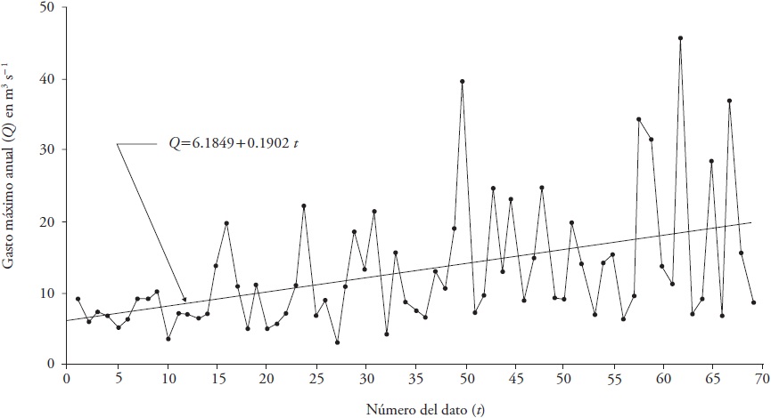
Figure 1 Linear trend l (upward) of the chronological series of the annual maximum flows (Q) in the hydrometric station of the River Aberjona, USA.
The second record, taken from Katz (2013), is an example of the drastic reduction of the maximum daily precipitation (PMD) in winter (May to October) recorded by the Manjimup station in the southwestern extreme of Australia. The record included 75 annual values (1930 to 2004), with a downward trend and greater variability at the beginning of the record (Figura 2).

Results and Discussion
Q Predictions in a station of the Aberjona River, USA
The data (Table 1) had an upward linear and significant trend, with statistics of the Student distribution of 3.850 and a critical value of 1.996 (p ≤ 0.05). The diagram of squared differences, between each data and the calculated linear trend showed that the variability was greater towards the end of the record (Figura 3).
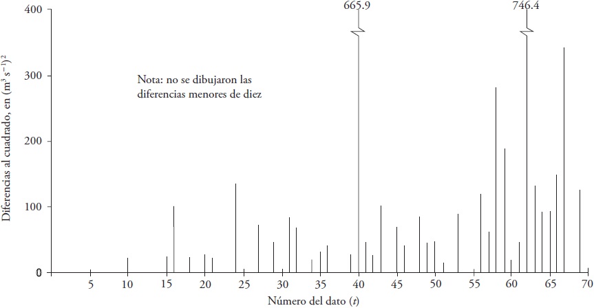
Figure 3 Differences (maximum annual flows minus the upward linear trend) to the square of the record of the hydrometric station of the Aberjona River, USA.
The linear model with the time t of the fit parameters u and a, leads to lower standard errors of fit (EEA) compared to those of the exponential model (Cuadro 2). With a mobile window width of 20 data, the lowest EEA was obtained, so these results were adopted to obtain predictions for the future (Figura 4).
Table 2 Non-stationary fit with mobile L-moments of the GVE11 distribution with window size of 15, 20, 25 and 30 maximum annual flow data of the Aberjona River, USA.
| Non-stationary fit (GVE11) with mobile window width (n) of 10 data | |||||
| nv = 59 | u m = 9.166 | a m = 5.005 | k m = -0.109 | ||
| Linear model with t | Exponential model with t | ||||
| α0 = 4.380 | α1 = 0.120 | ECM = 1.104 | γ0 = 5.226 | γ1 = 0.01325 | ECM = 1.116 |
| β0 = 0.957 | β1 = 0.101 | ECM = 1.344 | δ0 = 1.962 | δ1 = 0.02112 | ECM = 1.322 |
| EEA = 2.876 m-3·s | EEA = 3.103 m-3·s | ||||
| Non-stationary fit (GVE11) with mobile window width (n) of 15 data | |||||
| nv = 54 | u m = 8.990 | a m = 4.760 | k m = -0.175 | ||
| Linear model with t | Exponential model with t | ||||
| α0 = 4.209 | α1 = 0.112 | ECM = 0.620 | γ0 = 5.083 | γ1 = 0.01290 | ECM = 0.683 |
| β0 = 1.305 | β1 = 0.081 | ECM = 0.658 | δ0 = 2.001 | δ1 = 0.01915 | ECM = 0.740 |
| EEA = 2.330 m-3·s | EEA = 2.873 m-3·s | ||||
| Non-stationary fit (GVE11) with mobile window width (n) of 20 data | |||||
| nv = 49 | u m = 9.039 | a m = 4.745 | k m = -0.181 | ||
| Linear model with t | Exponential model with t | ||||
| α0 = 3.548 | α1 = 0.122 | ECM = 0.504 | γ0 = 4.720 | γ1 = 0.01398 | ECM = 0.584 |
| β0 = 1.298 | β1 = 0.077 | ECM = 0.581 | δ0 = 1.995 | δ1 = 0.01835 | ECM = 0.672 |
| EEA = 2.136 m-3·s | EEA = 2.473 m-3·s | ||||
| Non-stationary fit (GVE11) with mobile window width (n) of 25 data | |||||
| nv = 44 | u m = 9.093 | a m = 4.824 | k m = -0.176 | ||
| Linear model with t | Exponential model with t | ||||
| α0 = 2.892 | α1 = 0.131 | ECM = 0.394 | γ0 = 4.435 | γ1 = 0.0 | ECM = 0.448 |
| β0 = 1.078 | β1 = 0.079 | ECM = 0.486 | δ0 = 1.984 | δ1 = 0.01804 | ECM = 0.551 |
| EEA = 2.171 m-3·s | EEA = 2.241 m-3·s | ||||
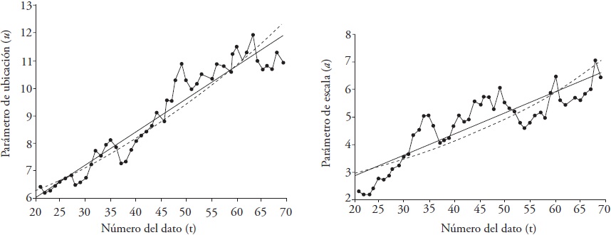
Figure 4 Linear (straight) and exponential (curve) trend of the location (u) and scale (a) parameters estimated with L-moments with 20 data in the width of the mobile window of the annual maximum flows of the Aberjona River, USA.
With the equations 11 to 15, the fit parameters of the stationary model (GVE0) were obtained: u = 8.407, a = 4.481 and k = -0.3034, with an EEA = 1.556 m3·s-1, and with equation 10 the predictions (Table 3). The non-stationary distribution GVE11 provided higher predictions in all return periods and even at the end of the historical record (Table 3). In the extreme periods of return (500 and 1000 years) and towards the year 2100, the predictions of the non-stationary model were twice those of the stationary model that did not consider the upward trend or the greater variability towards the end of the record.
Table 3 Predictions of maximum annual flow (m3·s-1) obtained with the distributions GVE0 and GVE11 with parameters u and a varying linearly and width of the mobile window of 20 data, in the Aberjona River, USA.
| Distributions GVE0 and GVE11 |
Return periods in years | |||||||
| 2 | 5 | 10 | 25 | 50 | 100 | 500 | 1000 | |
| Stationary | 10.1 | 16.9 | 22.9 | 32.6 | 41.9 | 53.3 | 90.9 | 113.7 |
| In the year 2008 | 14.5 | 23.3 | 30.2 | 40.5 | 49.3 | 59.2 | 87.4 | 102.4 |
| In the year 2025 | 17.0 | 27.6 | 35.9 | 48.2 | 58.7 | 70.6 | 104.5 | 122.3 |
| In the year 2050 | 20.8 | 34.0 | 44.3 | 59.5 | 72.6 | 87.3 | 129.5 | 151.7 |
| In the year 2100 | 28.4 | 46.7 | 61.0 | 82.2 | 100.4 | 120.9 | 179.5 | 210.4| |
PMD predictions in the Manjimup station of Australia
The annual daily maximum precipitation data (PMD) (Table 1) have a significant linear downward trend (Figure 2), with statistics of the Student distribution of -4.085 and critical value of 1.993 with p ≤ 0.05. In the diagram of squared differences, between each data and linear trend, the variability was noticeably higher at the beginning of the record (Figure 5).
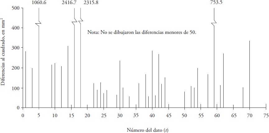
Figure 5 Differences (annual maximum daily precipitation minus the upward linear trend) to the square of the record of the pluviometric station Manjimup, Australia.
The exponential model with the time t of the fit parameters u and a, leads to lower standard errors of fit (EEA) compared with those of the linear model (Cuadro 4). As the size of the mobile window grows, lower EEAs are obtained, whereby those of the maximum proven value of n = 30 are adopted (Figura 6).
Table 4 Non-stationary fitting with mobile L-moments of the GVE11 distribution with window size of 15, 20, 25 and 30 annual PMD data from the Manjimup station, Australia.
| Non-stationary fit (GVE11) with mobile window width (n) of 15 data | |||||
| nv = 60 | u m = 36.930 | a m = 8.050 | k m = -0.009 | ||
| Linear model with t | Exponential model with t | ||||
| α0 = 48.982 | α1 = -0.265 | ECM = 3.410 | γ0 = 49.3973 | γ1 = -0.00690 | ECM = 3.253 |
| β0 = 14.124 | β1 = -0.134 | ECM = 1.670 | δ0 = 15.684 | δ1 = -0.01606 | ECM = 1.536 |
| EEA = 12.804 mm | EEA = 12.176 mm | ||||
| Non-stationary fit (GVE11) with mobile window width (n) of 20 data | |||||
| nv = 55 | u m = 36.292 | a m = 7.828 | k m = -0.072 | ||
| Linear model with t | Exponential model with t | ||||
| α0 = 49.933 | α1 = -0.284 | ECM = 2.949 | γ0 = 51.545 | γ1 = -0.00753 | ECM = 2.773 |
| β0 = 14.137 | β1 = -0.131 | ECM = 1.378 | δ0 = 16.183 | δ1 = -0.01620 | ECM = 1.255 |
| EEA = 12.472 mm | EEA = 11.898 mm | ||||
| Non-stationary fit (GVE11) with mobile window width (n) of 25 data | |||||
| nv = 50 | u m = 35.733 | a m = 7.647 | k m = -0.105 | ||
| Linear model with t | Exponential model with t | ||||
| α0 = 50.660 | α1 = -0.296 | ECM = 2.528 | γ0 = 52.906 | γ1 = -0.00795 | ECM = 2.351 |
| β0 = 14.867 | β1 = -0.143 | ECM = 1.023 | δ0 = 18.459 | δ1 = -0.01835 | ECM = 0.923 |
| EEA = 12.427 mm | EEA = 11.826 mm | ||||
| Non-stationary fit (GVE11) with mobile window width (n) of 30 data | |||||
| nv = 45 | u m = 35.275 | a m = 7.666 | k m = -.120 | ||
| Linear model with t | Exponential model with t | ||||
| α0 = 50.327 | α1 = -0.284 | ECM = 1.904 | γ0 = 52.923 | γ1 = -0.00778 | ECM = 1.761 |
| β0 = 15.864 | β1 = -0.155 | ECM = 0.800 | δ0 = 21.281 | δ1 = -0.02000 | ECM = 0.731 |
| EEA = 11.777 mm | EEA = 11.199 mm | ||||
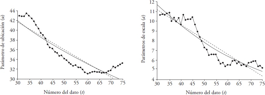
Figure 6 Linear (straight) and exponential (curve) trend of the location (u) and scale (a) parameters estimated with L-moments with 30 data in the width of the mobile window in the annual PMD of the Manjimup station, Australia.
Based on equations 11 to 15, the fit parameters of the stationary model GVE0 were obtained: u = 35.488, a = 8.431 and k = -0.1846, with an EEA = 2.881 mm. The respective predictions, obtained with equation 10, showed that the non-stationary distribution GVE11 contributed lower predictions, from the end of the historical record and in all the return periods analyzed (Cuadro 5). In the extreme return periods analyzed (500 and 1000 years) and towards the year 2100, predictions of PMD tended to stabilize around 21 mm.
Table 5 Predictions of PMD obtained with the stationary GVE and non-stationary (GVE11) distributions with parameters varying exponentially and width of the mobile window (n) of 30 data, at the Manjimup station, Australia.
| Distributions GVE0 and GVE11 |
Return periods in years | |||||||
| 2 | 5 | 10 | 25 | 50 | 100 | 500 | 1000 | |
| Stationary | 38.7 | 50.1 | 59.0 | 72.2 | 83.7 | 96.6 | 133.6 | 153.3 |
| In the year 2004 | 31.3 | 37.3 | 41.8 | 48.0 | 53.1 | 58.7 | 73.3 | 80.6 |
| In the year 2025 | 26.3 | 30.2 | 33.1 | 37.3 | 40.6 | 44.2 | 53.9 | 58.6 |
| In the year 2050 | 21.4 | 23.8 | 25.5 | 28.0 | 30.1 | 32.3 | 38.1 | 41.0 |
| In the year 2100 | 14.3 | 15.1 | 15.8 | 16.7 | 17.5 | 18.3 | 20.4 | 21.5 |
Applicability of the mobile L-moments method
The linear representation of both parameters and significantly better of the location parameter (u) is acceptable for the Aberjona River, USA (Figure 4). At the Manjimup station, Australia (Figure 6) the scale parameter representation (a) may be acceptable, but the one relative to the location parameter u may be not acceptable.
The higher statistical quality of the fit with the mobile L-moments method is numerically highlighted because of the similarity shown by the standard errors of fit (EEA) of the stationary (GVE0) and non-stationary (GVE11) models. In the case of the Aberjona River, USA, the EEA of the stationary and non-stationary GVE were 1.556 and 2.136 m3·s-1, that is, with an order of similar magnitude. In contrast, at the Manjimup station, Australia, the EEA of both models (2.881 and 11.199 mm) were different and much greater that of the GVE11 distribution, therefore, is not acceptable to the PMD data group.
Conclusions
The method of the mobile L-moments (MLM) proposed by Cunderlik and Burn (2003) and applied by Mudersbach and Jensen (2010 a, b), for the fit of the GVE11 distribution, with variable location and scale parameters, linear or exponential with the covariate time, is a practical procedure, recommended for the hydrological analysis of annual maximum data frequencies that present changing trends and variability through their record, which must be large. The use of different sizes of the mobile window is suggested in the operating procedure of the MLM method, to fit according to each one the GVE11 distribution, selecting the most convenient to the record processed through the lowest standard error of fit.
The statistical convenience or goodness of fit of the MLM method to the processed non-stationary record is judged through the linear or exponential representativeness of the chronological series of the location, scale parameters calculated as well as the numerical similarity that has the standard error of fit of the GVE0 and GVE11 distributions.
With two numerical applications the simplicity of the MLM method is demonstrated and, based on the predictions, its importance and usefulness are highlighted, in the probabilistic analyses of large records of extreme hydrological data that exhibit non-constant tendency and variability.
Literatura Citada
Aissaoui-Fqayeh, I., S. El Adlouni, T. B. M. J. Ouarda, and A. St-Hilaire. 2009. Développement du modèle log-normal non-stationnaire et comparaison avec le modèle GEV non-stationnaire. Hydrol. Sci. J. 54: 1141-1156. [ Links ]
Al Saji, M., J. J. O’Sullivan, and A. O’Connor. 2015. Design impact and significance of non-stationary of variance in extreme rainfall. Proc. IAHS, No. 371, pp: 117-123. [ Links ]
Álvarez-Olguín, G., y C. A. Escalante-Sandoval. 2016. Análisis de frecuencias no estacionario de series de lluvia anual. Tecnol. Cienc. Agua VII: 71-88. [ Links ]
Asquith, W. H. 2011. Probability-weighted moments. In: Distributional Analysis with L-moment Statistics using the R Environment for Statistical Computing. Author edition (ISBN-13: 978-1463508418). Texas, U.S.A. pp: 77-86. [ Links ]
Benson, M. A. 1962. Plotting positions and economics of engineering planning. J. Hydraulics Div. 88: 57-71. [ Links ]
Campos-Aranda, D. F. 2015. Búsqueda del cambio climático en la temperatura máxima de mayo en 16 estaciones climatológicas del estado de Zacatecas, México. Tecnol. Cienc. Agua VI: 143-160. [ Links ]
Campos-Aranda, D. F. 2016.Ajuste de las distribuciones GVE, LOG y PAG con momentos L de orden mayor. Ing. Invest. Tecnol. XVII: 131-142. [ Links ]
Cunderlik, J. M. and D. H. Burn. 2003. Non-stationary pooled flood frequency analysis. J Hydrol. 276: 210-223.7 [ Links ]
Davis, P. J. 1972. Gamma Function and related functions. In: Abramowitz M. and I. Stegun (eds). Handbook of Mathematical Functions. Dover Publications. New York, U.S.A. Ninth printing. pp: 253-296. [ Links ]
El Adlouni, S., T. B. M. J. Ouarda, X. Zhang, R. Roy, and B. Bobée. 2007. Generalized maximum likelihood estimators for the nonstationary generalized extreme value model. Water Resour. Res. 43: 1-13 (W03410). [ Links ]
El Adlouni, S., B. Bobée, and T. B. M. J. Ouarda. 2008. On the tails of extreme event distributions in hydrology. J. Hydrol. 355: 16-33. [ Links ]
Franks, S. W., C. J. White and M. Gensen. 2015. Estimating extreme flood events-assumptions, uncertainty and error. Proc. IAHS, No. 369, pp: 31-36. [ Links ]
Greenwood, J. A., J. M. Landwehr, N. C. Matalas, and J. R. Wallis. 1979. Probability weighted moments: Definition and relation to parameters of several distributions expressible in inverse form. Water Resour. Res. 15: 1049-1054. [ Links ]
Hosking, J. R. M. 1990. L-moments: analysis and estimation of distributions using linear combinations of order statistics. J. R. Stat. Soc. Ser. B, 52: 105-124. [ Links ]
Hosking, J. R. M., and J. R. Wallis. 1997. Regional Frequency Analysis. An Approach based on L-moments. Cambridge University Press. Cambridge, England. 224 p. [ Links ]
Jakob, D. 2013. Nonstationarity in extremes and engineering design. In: AghaKouchak, A., D. Easterling, K. Hsu, S. Schubert, and S. Sorooshian (eds). Extremes in a Changing Climate. Springer. Dordrecht, The Netherlands. pp: 393-417. [ Links ]
Katz, R. W. 2013. Statistical methods for nonstationary extremes. In: AghaKouchak, A., D. Easterling, K. Hsu, S. Schubert and S. Sorooshian (eds). Extremes in a Changing Climate. Springer. Dordrecht, The Netherlands. pp: 15-37. [ Links ]
Khaliq, M. N., T. B. M. J. Ouarda, J. C. Ondo, P. Gachon, and B. Bobée. 2006. Frequency analysis of a sequence of dependent and/or non-stationary hydro-meteorological observations: A review. J. Hydrol. 329: 534-552. [ Links ]
Kim, S., W. Nam , H. Ahn, T. Kim, and J. H. Heo. 2015. Comparison of nonstationary generalized logistic models based on Monte Carlo simulation. Proc. IAHS, No. 371, pp: 65-68. [ Links ]
Kite, G. W. 1977. Comparison of frequency distributions. In: Frequency and Risk Analyses in Hydrology. Water Resources Publications. Fort Collins, Colorado, U.S.A. pp: 156-168. [ Links ]
Meylan, P., A. C. Fabre, and A. Musy. 2012. Predictive Hydrology. A Frequency Analysis Approach. CRC Press. Boca Raton, Florida, U.S.A. 212 p. [ Links ]
Mudersbach, C., and J. Jensen. 2010a. Nonstationary extreme value analysis of annual maximum water levels for designing coastal structures on the German North Sea coastline. J. Flood Risk Manag. 3: 52-62. [ Links ]
Mudersbach, C., and J. Jensen. 2010b. An advanced statistical extreme value model for evaluating storm surge heights considering systematic records and sea level scenarios. In: Proc. 32nd Conference on Coastal Engineering. Shanghai, China. pp: currents 23. [ Links ]
Pandey, G. R., and V. T. V. Nguyen. 1999. A comparative study of regression based methods in regional flood frequency analysis. J. Hydrol. 225: 92-101. [ Links ]
Park, J. S., H. S. Kang, Y. S. Lee, and M. K. Kim. 2011. Changes in the extreme daily rainfall in South Korea. Int. J. Climatol. 31: 2290-2299. [ Links ]
Rao, A. R. and K. H. Hamed. 2000. Flood Frequency Analysis. CRC Press. Boca Raton, Florida, U.S.A. 350 p. [ Links ]
Stedinger, J. R., R. M. Vogel, and E. Foufoula-Georgiou. 1993. Frequency analysis of extreme events. In: Maidment, D. R. (ed). Handbook of Hydrology. McGraw-Hill, Inc. New York, U.S.A. pp: 18.1-18.66. [ Links ]
Vogel, R. M., C. Yaindl, and M. Walter. 2011. Nonstationarity: Flood magnification and recurrence reduction factors in the United States. J. Am. Water Resour. Assoc. 47: 464-474. [ Links ]
Wang, Q. J. 1997. LH moments for statistical analysis of extreme events. Water Resour. Res. 33: 2841-2848. [ Links ]
Received: November 2017; Accepted: January 2018
 Este es un artículo publicado en acceso abierto bajo una licencia Creative Commons
